Solving positive definite linear systems

This benchmark compares the performances of KeOps versus Numpy and Pytorch on a inverse matrix operation. It uses the functions torch.KernelSolve (see also here) and numpy.KernelSolve (see also here).

In a nutshell, given $$\begin{gathered} x\in {\mathbb{R}}^{N \\ timesD} \end{gathered}$$ and $$\begin{gathered} b\in {\mathbb{R}}^{N \\ times{D}_v} \end{gathered}$$, we compute $$\begin{gathered} a\in {\mathbb{R}}^{N \\ times{D}_v} \end{gathered}$$ so that

$$\begin{array}{r}b=(\\ alpha\mathrm{Id}+K_{x,x})a\iff a=(\\ alpha\mathrm{Id}+K_{x,x}{)}^{-1}b\end{array}$$

where $K_{x,x}=[\exp (-\Vert x_i-x_j{\Vert }^2/{\sigma }^2){]}_{i,j=1}^N$. The method is based on a conjugate gradient scheme. The benchmark tests various values of $N\in [10,\cdots ,{10}^6]$.

Note

In this demo, we implement the linear operator $K_{x}x$ using a bruteforce implementation and do not leverage any multiscale or low-rank (Nystroem/multipole) decomposition of the Kernel matrix. Going further, advanced strategies and solvers are now available through the GPyTorch and Falkon libraries, which rely on a KeOps backend whenever relevant.

Setup

Standard imports:

import numpy as np
import torch
from matplotlib import pyplot as plt

from scipy.sparse import diags
from scipy.sparse.linalg import aslinearoperator, cg

from pykeops.numpy import KernelSolve as KernelSolve_np, LazyTensor
from pykeops.torch import KernelSolve
from pykeops.torch.utils import squared_distances as sqdist_torch
from pykeops.numpy.utils import squared_distances as sqdist_np

from benchmark_utils import flatten, random_normal, unit_tensor, full_benchmark

use_cuda = torch.cuda.is_available()

if torch.__version__ >= "1.8":
    torchsolve = lambda A, B: torch.linalg.solve(A, B)
else:
    torchsolve = lambda A, B: torch.solve(B, A)[0]

Benchmark specifications:

D = 3  # Let's do this in 3D
Dv = 1  # Dimension of the vectors (= number of linear problems to solve)

# Numbers of samples that we'll loop upon:
problem_sizes = flatten(
    [[1 * 10**k, 2 * 10**k, 5 * 10**k] for k in [1, 2, 3, 4, 5]] + [[10**6]]
)
D = 3  # We work with 3D points
Dv = 1  # and solve one problem at a time.

Create some random input data:

def generate_samples(N, device="cuda", lang="torch", **kwargs):
    """Generates a point cloud x, a scalar signal b of size N and two regularization parameters.

    Args:
        N (int): number of point.
        device (str, optional): "cuda", "cpu", etc. Defaults to "cuda".
        lang (str, optional): "torch", "numpy", etc. Defaults to "torch".

    Returns:
        3-uple of arrays: x, y, b
    """
    randn = random_normal(device=device, lang=lang)
    ones = unit_tensor(device=device, lang=lang)

    x = randn((N, D))
    b = randn((N, Dv))
    gamma = ones((1,)) / (2 * 0.01**2)  # kernel bandwidth
    alpha = ones((1,)) * 0.8  # regularization
    return x, b, gamma, alpha

KeOps kernel

Define a Gaussian RBF kernel:

formula = "Exp(- g * SqDist(x,y)) * a"
aliases = [
    "x = Vi(" + str(D) + ")",  # First arg:  i-variable of size D
    "y = Vj(" + str(D) + ")",  # Second arg: j-variable of size D
    "a = Vj(" + str(Dv) + ")",  # Third arg:  j-variable of size Dv
    "g = Pm(1)",
]  # Fourth arg: scalar parameter

Note

This operator uses a conjugate gradient solver and assumes that formula defines a symmetric, positive and definite linear reduction with respect to the alias "a" specified trough the third argument.

Define the Kernel solver, with a ridge regularization alpha:

def Kinv_keops(x, b, gamma, alpha, **kwargs):
    Kinv = KernelSolve(formula, aliases, "a", axis=1)
    res = Kinv(x, x, b, gamma, alpha=alpha)
    return res


def Kinv_keops_numpy(x, b, gamma, alpha, **kwargs):
    Kinv = KernelSolve_np(formula, aliases, "a", axis=1, dtype="float32")
    res = Kinv(x, x, b, gamma, alpha=alpha)
    return res


def Kinv_scipy(x, b, gamma, alpha, **kwargs):
    x_i = LazyTensor(np.sqrt(gamma) * x[:, None, :])
    y_j = LazyTensor(np.sqrt(gamma) * x[None, :, :])

    K_ij = (-((x_i - y_j) ** 2).sum(2)).exp()

    A = aslinearoperator(diags(alpha * np.ones(x.shape[0]))) + aslinearoperator(K_ij)
    A.dtype = np.dtype("float32")
    res = cg(A, b)
    return res

Define the same Kernel solver, using a tensorized implementation:

def Kinv_pytorch(x, b, gamma, alpha, **kwargs):
    K_xx = alpha * torch.eye(x.shape[0], device=x.get_device()) + torch.exp(
        -gamma * sqdist_torch(x, x)
    )
    res = torchsolve(K_xx, b)
    return res


def Kinv_numpy(x, b, gamma, alpha, **kwargs):
    K_xx = alpha * np.eye(x.shape[0]) + np.exp(-gamma * sqdist_np(x, x))
    res = np.linalg.solve(K_xx, b)
    return res

Run the benchmark

routines = [
    (Kinv_numpy, "NumPy", {"lang": "numpy"}),
    (Kinv_pytorch, "PyTorch", {}),
    (Kinv_keops_numpy, "NumPy + KeOps", {"lang": "numpy"}),
    (Kinv_keops, "PyTorch + KeOps", {}),
    (Kinv_scipy, "Scipy + KeOps", {"lang": "numpy"}),
]
full_benchmark(
    "Inverse radial kernel matrix",
    routines,
    generate_samples,
    problem_sizes=problem_sizes,
    max_time=1,
)

plt.show()

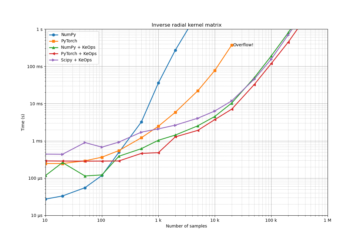
Benchmarking : Inverse radial kernel matrix ===============================
NumPy -------------
  1x100 loops of size   10 :   1x100x  27.3 µs
  1x100 loops of size   20 :   1x100x  33.2 µs
  1x100 loops of size   50 :   1x100x  55.3 µs
  1x100 loops of size  100 :   1x100x 117.8 µs
  1x100 loops of size  200 :   1x100x 495.0 µs
  1x100 loops of size  500 :   1x100x   3.2 ms
  1x100 loops of size   1 k:   1x100x  35.6 ms
  1x 10 loops of size   2 k:   1x 10x 271.9 ms
  1x  1 loops of size   5 k:   1x  1x    2.7 s
** Too slow!
PyTorch -------------
  1x100 loops of size   10 :   1x100x 245.9 µs
  1x100 loops of size   20 :   1x100x 246.4 µs
  1x100 loops of size   50 :   1x100x 290.7 µs
  1x100 loops of size  100 :   1x100x 364.6 µs
  1x100 loops of size  200 :   1x100x 548.8 µs
  1x100 loops of size  500 :   1x100x   1.2 ms
  1x100 loops of size   1 k:   1x100x   2.5 ms
  1x100 loops of size   2 k:   1x100x   5.9 ms
  1x100 loops of size   5 k:   1x100x  22.0 ms
  1x 10 loops of size  10 k:   1x 10x  77.1 ms
  1x 10 loops of size  20 k:   1x 10x 372.6 ms
CUDA out of memory. Tried to allocate 9.31 GiB. GPU 0 has a total capacity of 23.68 GiB of which 3.35 GiB is free. Including non-PyTorch memory, this process has 20.30 GiB memory in use. Of the allocated memory 18.64 GiB is allocated by PyTorch, and 23.12 MiB is reserved by PyTorch but unallocated. If reserved but unallocated memory is large try setting PYTORCH_CUDA_ALLOC_CONF=expandable_segments:True to avoid fragmentation.  See documentation for Memory Management  (https://pytorch.org/docs/stable/notes/cuda.html#environment-variables)
** Runtime error!
NumPy + KeOps -------------
  1x100 loops of size   10 :   1x100x 117.2 µs
  1x100 loops of size   20 :   1x100x 261.5 µs
  1x100 loops of size   50 :   1x100x 114.3 µs
  1x100 loops of size  100 :   1x100x 121.7 µs
  1x100 loops of size  200 :   1x100x 386.8 µs
  1x100 loops of size  500 :   1x100x 617.1 µs
  1x100 loops of size   1 k:   1x100x   1.0 ms
  1x100 loops of size   2 k:   1x100x   1.4 ms
  1x100 loops of size   5 k:   1x100x   2.5 ms
  1x100 loops of size  10 k:   1x100x   4.5 ms
  1x100 loops of size  20 k:   1x100x  10.4 ms
  1x 10 loops of size  50 k:   1x 10x  49.2 ms
  1x 10 loops of size 100 k:   1x 10x 188.9 ms
  1x  1 loops of size 200 k:   1x  1x 794.8 ms
  1x  1 loops of size 500 k:   1x  1x    6.2 s
** Too slow!
PyTorch + KeOps -------------
  1x100 loops of size   10 :   1x100x 289.3 µs
  1x100 loops of size   20 :   1x100x 286.6 µs
  1x100 loops of size   50 :   1x100x 284.5 µs
  1x100 loops of size  100 :   1x100x 286.2 µs
  1x100 loops of size  200 :   1x100x 288.7 µs
  1x100 loops of size  500 :   1x100x 460.4 µs
  1x100 loops of size   1 k:   1x100x 481.3 µs
  1x100 loops of size   2 k:   1x100x   1.3 ms
  1x100 loops of size   5 k:   1x100x   1.9 ms
  1x100 loops of size  10 k:   1x100x   3.7 ms
  1x100 loops of size  20 k:   1x100x   7.1 ms
  1x100 loops of size  50 k:   1x100x  32.3 ms
  1x 10 loops of size 100 k:   1x 10x 117.9 ms
  1x  1 loops of size 200 k:   1x  1x 443.2 ms
  1x  1 loops of size 500 k:   1x  1x    3.2 s
** Too slow!
Scipy + KeOps -------------
  1x100 loops of size   10 :   1x100x 441.3 µs
  1x100 loops of size   20 :   1x100x 436.2 µs
  1x100 loops of size   50 :   1x100x 900.1 µs
  1x100 loops of size  100 :   1x100x 678.0 µs
  1x100 loops of size  200 :   1x100x 927.3 µs
  1x100 loops of size  500 :   1x100x   1.7 ms
  1x100 loops of size   1 k:   1x100x   2.1 ms
  1x100 loops of size   2 k:   1x100x   2.6 ms
  1x100 loops of size   5 k:   1x100x   4.0 ms
  1x100 loops of size  10 k:   1x100x   6.3 ms
  1x100 loops of size  20 k:   1x100x  11.8 ms
  1x 10 loops of size  50 k:   1x 10x  45.1 ms
  1x 10 loops of size 100 k:   1x 10x 155.2 ms
  1x  1 loops of size 200 k:   1x  1x 692.8 ms
  1x  1 loops of size 500 k:   1x  1x    5.2 s
** Too slow!