KernelSolve reduction

Let’s see how to solve discrete deconvolution problems using the conjugate gradient solver provided by numpy.KernelSolve.

Setup

Standard imports:

import numpy as np
import time
import matplotlib.pyplot as plt

from pykeops.numpy import KernelSolve
import pykeops.config

Define our dataset:

N = 5000 if pykeops.config.gpu_available else 500  # Number of points
D = 2  # Dimension of the ambient space
Dv = 2  # Dimension of the vectors (= number of linear problems to solve)
sigma = 0.1  # Radius of our RBF kernel

dtype = "float32"
x = np.random.rand(N, D).astype(dtype)
b = np.random.rand(N, Dv).astype(dtype)
g = np.array([0.5 / sigma**2]).astype(dtype)  # Parameter of the Gaussian RBF kernel

KeOps kernel

Define a Gaussian RBF kernel:

formula = "Exp(- g * SqDist(x,y)) * b"
aliases = [
    "x = Vi(" + str(D) + ")",  # First arg:  i-variable of size D
    "y = Vj(" + str(D) + ")",  # Second arg: j-variable of size D
    "b = Vj(" + str(Dv) + ")",  # Third arg:  j-variable of size Dv
    "g = Pm(1)",
]  # Fourth arg: scalar parameter

Define the inverse kernel operation, with a ridge regularization alpha:

alpha = 0.01
Kinv = KernelSolve(formula, aliases, "b", axis=1, dtype=dtype)

Note

This operator uses a conjugate gradient solver and assumes that formula defines a symmetric, positive and definite linear reduction with respect to the alias "b" specified trough the third argument.

Apply our solver on arbitrary point clouds:

# Warmup of gpu
Kinv(x, x, b, g, alpha=alpha)

print("Solving a Gaussian linear system, with {} points in dimension {}.".format(N, D))
start = time.time()
c = Kinv(x, x, b, g, alpha=alpha)
end = time.time()
print("Timing (KeOps implementation):", round(end - start, 5), "s")

Solving a Gaussian linear system, with 5000 points in dimension 2.
Timing (KeOps implementation): 0.17704 s

Compare with a straightforward Numpy implementation:

start = time.time()
K_xx = alpha * np.eye(N) + np.exp(
    -g * np.sum((x[:, None, :] - x[None, :, :]) ** 2, axis=2)
)
c_np = np.linalg.solve(K_xx, b)
end = time.time()
print("Timing (Numpy implementation):", round(end - start, 5), "s")
print("Relative error = ", np.linalg.norm(c - c_np) / np.linalg.norm(c_np))

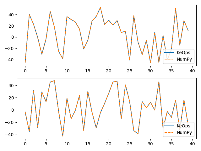
# Plot the results next to each other:
for i in range(Dv):
    plt.subplot(Dv, 1, i + 1)
    plt.plot(c[:40, i], "-", label="KeOps")
    plt.plot(c_np[:40, i], "--", label="NumPy")
    plt.legend(loc="lower right")
plt.tight_layout()
plt.show()

Timing (Numpy implementation): 0.81175 s
Relative error =  9.646320829943949e-05