KernelSolve reduction

Let’s see how to solve discrete deconvolution problems using the conjugate gradient solver provided by pykeops.torch.KernelSolve.

Setup

Standard imports:

import time

import torch
from matplotlib import pyplot as plt

from pykeops.torch import KernelSolve

if torch.__version__ >= "1.8":
    torchsolve = lambda A, B: torch.linalg.solve(A, B)
else:
    torchsolve = lambda A, B: torch.solve(B, A)[0]

Define our dataset:

N = 5000 if torch.cuda.is_available() else 500  # Number of points
D = 2  # Dimension of the ambient space
Dv = 2  # Dimension of the vectors (= number of linear problems to solve)
sigma = 0.1  # Radius of our RBF kernel

x = torch.rand(N, D, requires_grad=True)
b = torch.rand(N, Dv)
g = torch.Tensor([0.5 / sigma**2])  # Parameter of the Gaussian RBF kernel

if torch.cuda.is_available():
    sync = torch.cuda.synchronize
else:

    def sync():
        pass

KeOps kernel

Define a Gaussian RBF kernel:

formula = "Exp(- g * SqDist(x,y)) * b"
aliases = [
    "x = Vi(" + str(D) + ")",  # First arg:  i-variable of size D
    "y = Vj(" + str(D) + ")",  # Second arg: j-variable of size D
    "b = Vj(" + str(Dv) + ")",  # Third arg:  j-variable of size Dv
    "g = Pm(1)",
]  # Fourth arg: scalar parameter

Define the inverse kernel operation, with a ridge regularization alpha:

alpha = 0.01
Kinv = KernelSolve(formula, aliases, "b", axis=1)

Note

This operator uses a conjugate gradient solver and assumes that formula defines a symmetric, positive and definite linear reduction with respect to the alias "b" specified trough the third argument.

Apply our solver on arbitrary point clouds:

print("Solving a Gaussian linear system, with {} points in dimension {}.".format(N, D))
sync()
start = time.time()
c = Kinv(x, x, b, g, alpha=alpha)
sync()
end = time.time()
print("Timing (KeOps implementation):", round(end - start, 5), "s")

Solving a Gaussian linear system, with 5000 points in dimension 2.
Timing (KeOps implementation): 0.20262 s

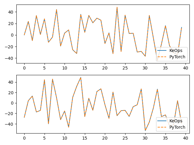
Compare with a straightforward PyTorch implementation:

sync()
start = time.time()
K_xx = alpha * torch.eye(N) + torch.exp(
    -torch.sum((x[:, None, :] - x[None, :, :]) ** 2, dim=2) / (2 * sigma**2)
)
c_py = torchsolve(K_xx, b)
sync()
end = time.time()
print("Timing (PyTorch implementation):", round(end - start, 5), "s")
print("Relative error = ", (torch.norm(c - c_py) / torch.norm(c_py)).item())


# Plot the results next to each other:
for i in range(Dv):
    plt.subplot(Dv, 1, i + 1)
    plt.plot(c.cpu().detach().numpy()[:40, i], "-", label="KeOps")
    plt.plot(c_py.cpu().detach().numpy()[:40, i], "--", label="PyTorch")
    plt.legend(loc="lower right")
plt.tight_layout()
plt.show()

Timing (PyTorch implementation): 0.21693 s
Relative error =  0.0004108477442059666

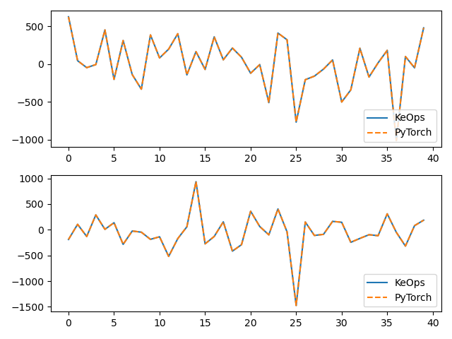
Compare the derivatives:

print("1st order derivative")
e = torch.randn(N, D)
start = time.time()
(u,) = torch.autograd.grad(c, x, e)
end = time.time()
print("Timing (KeOps derivative):", round(end - start, 5), "s")
start = time.time()
(u_py,) = torch.autograd.grad(c_py, x, e)
end = time.time()
print("Timing (PyTorch derivative):", round(end - start, 5), "s")
print("Relative error = ", (torch.norm(u - u_py) / torch.norm(u_py)).item())


# Plot the results next to each other:
for i in range(Dv):
    plt.subplot(Dv, 1, i + 1)
    plt.plot(u.cpu().detach().numpy()[:40, i], "-", label="KeOps")
    plt.plot(u_py.cpu().detach().numpy()[:40, i], "--", label="PyTorch")
    plt.legend(loc="lower right")
plt.tight_layout()
plt.show()

1st order derivative
Timing (KeOps derivative): 0.2239 s
Timing (PyTorch derivative): 0.15306 s
Relative error =  0.001857273979112506