Anisotropic kernels

Let’s see how to encode anisotropic kernels with a minimal amount of effort.

Setup

Standard imports:

import numpy as np
from matplotlib import pyplot as plt
import matplotlib.cm as cm
import torch
from pykeops.torch import Vi, Vj, Pm, LazyTensor

Dataset:

# Choose the storage place for our data : CPU (host) or GPU (device) memory.
dtype = torch.cuda.FloatTensor if torch.cuda.is_available() else torch.FloatTensor

# Three points in the plane R^2
y = torch.tensor([[0.2, 0.7], [0.5, 0.3], [0.7, 0.5]]).type(dtype)

# Three scalar weights
b = torch.tensor([1.0, 1.0, 0.5]).type(dtype)

# Remember that KeOps is super-picky on the input shapes:
# b is not a vector, but a 'list of unidimensional vectors'!
b = b.view(-1, 1)

# Create a uniform grid on the unit square:
res = 100
ticks = np.linspace(0, 1, res + 1)[:-1] + 0.5 / res
X, Y = np.meshgrid(ticks, ticks)

# Beware! By default, numpy uses float64 precision whereas pytorch uses float32.
# If you don't convert explicitely your data to compatible dtypes,
# PyTorch or Keops will throw an error.
x = torch.from_numpy(np.vstack((X.ravel(), Y.ravel())).T).contiguous().type(dtype)

Kernel definition

Let’s use a Gaussian kernel given through

\[k(x_i,y_j) = \exp( -\|x - y\|_{\Gamma}^2) = \exp( - (x_i - y_j)^t \Gamma (x_i-y_j) ),\]

which is equivalent to the KeOps formula exp(-WeightedSquareNorm(gamma, x_i-y_j )). Using the high-level pykeops.torch.LazyTensor, we can simply define:

def plot_kernel(gamma):
    """Samples 'x -> ∑_j b_j * k_j(x - y_j)' on the grid, and displays it as a heatmap."""
    if gamma.dim() == 2:
        heatmap = (-Vi(x).weightedsqdist(Vj(y), Vj(gamma))).exp() @ b
    else:
        heatmap = (-Vi(x).weightedsqdist(Vj(y), Pm(gamma))).exp() @ b
    heatmap = heatmap.view(res, res).cpu().numpy()  # reshape as a 'background' image
    plt.imshow(
        -heatmap,
        interpolation="bilinear",
        origin="lower",
        vmin=-1,
        vmax=1,
        cmap=cm.RdBu,
        extent=(0, 1, 0, 1),
    )
    plt.show()

The precise meaning of the computation is then defined through the entry gamma, which will is to be used as a ‘metric multiplier’. Denoting D == x.shape[1] == y.shape[1] the size of the feature space, the integer K can be 1, D or D*D. Rules are:

• if gamma is a vector (gamma.shape = [K]), it is seen as a fixed parameter

• if gamma is a 2d-tensor (gamma.shape = [M,K]), it is seen as a j-variable

N.B.: Beware of Shape([K]) != Shape([1,K]) confusions!

Isotropic Kernels

If K == 1 (ie gamma is a float): \(\Gamma = \gamma Id_D\) is a scalar factor in front of a simple Euclidean squared norm. In this case, WeightedSquareNorm(gamma, x-y ) corresponds to

\[\|x - y\|_{\Gamma}^2 = \gamma \|x-y\|^2\]

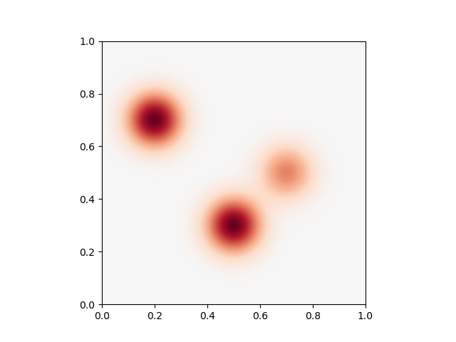
Uniform kernels

Providing a single scalar we get uniform kernels

sigma = torch.tensor([0.1]).type(dtype)
gamma = 1.0 / sigma**2
plt.plot()
plot_kernel(gamma)

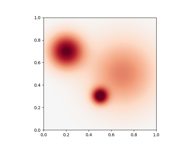
Variable kernels

Providing a list of scalar we get variable kernels

sigma = torch.tensor([[0.15], [0.07], [0.3]]).type(dtype)
gamma = 1.0 / sigma**2
plot_kernel(gamma)

Diagonal Kernels

If K == D (ie gamma is a vector): \(\Gamma = \text{diag}(\gamma)\) is a diagonal matrix. In that case, WeightedSquareNorm(gamma, x-y) corresponds to

\[\|x - y\|_{\Gamma}^2 = \langle (x-y), \Gamma (x-y) \rangle = \langle (x-y), \text{diag}(\gamma) (x-y) \rangle = \sum_d \gamma_d (x_d-y_d)^2\]

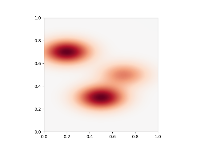
Uniform kernels

Providing a single vector we get uniform kernels

sigma = torch.tensor([0.2, 0.1]).type(dtype)
gamma = 1.0 / sigma**2
plot_kernel(gamma)

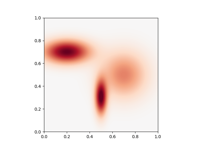
Variable kernels

Providing a list of vector (ie a 2d-tensor) we get variable kernels

sigma = torch.tensor([[0.2, 0.1], [0.05, 0.15], [0.2, 0.2]]).type(dtype)
gamma = 1.0 / sigma**2
plot_kernel(gamma)

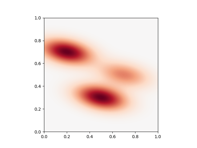
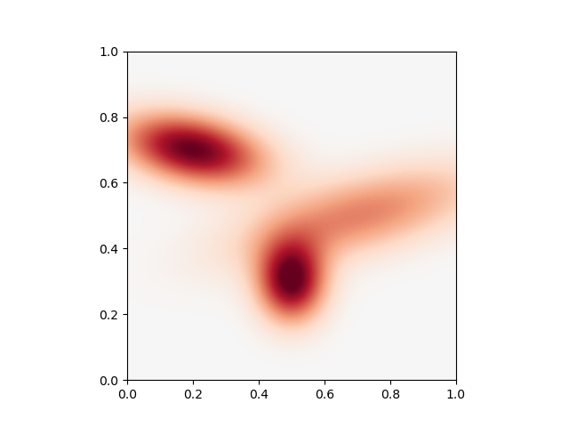
Fully-Anisotropic kernels

If K == D*D (ie gamma is a vector of size the dimension of the ambiant space squared): \(\Gamma\) is a symmetric matrix whose entries are stored in \(\gamma\). In that case, WeightedSquareNorm(gamma, x-y) corresponds to

\[\|x - y\|_{\Gamma}^2 = \langle (x-y), \Gamma (x-y) \rangle = \sum_{k}\sum_{\ell} g_{k,\ell} (x_k-y_k)(x_\ell-y_\ell) )\]

Uniform kernels

Providing a single vector we get uniform kernels

Sigma = torch.tensor([1 / 0.2**2, 1 / 0.25**2, 1 / 0.25**2, 1 / 0.1**2]).type(dtype)
gamma = Sigma
plot_kernel(gamma)

Variable kernels

Providing a list of vector (ie a 2d-tensor) we get variable kernels

Sigma = torch.tensor(
    [
        [1 / 0.2**2, 1 / 0.25**2, 1 / 0.25**2, 1 / 0.1**2],
        [1 / 0.1**2, 0, 0, 1 / 0.12**2],
        [1 / 0.3**2, -1 / 0.25**2, -1 / 0.25**2, 1 / 0.12**2],
    ]
).type(dtype)

gamma = Sigma
# sphinx_gallery_thumbnail_number = 6
plot_kernel(gamma)