Note
Click here to download the full example code
Sampling on the Poincare disk
Let’s illustrate the versatility of our toolbox by sampling an arbitrary distribution in the hyperbolic plane.
Introduction
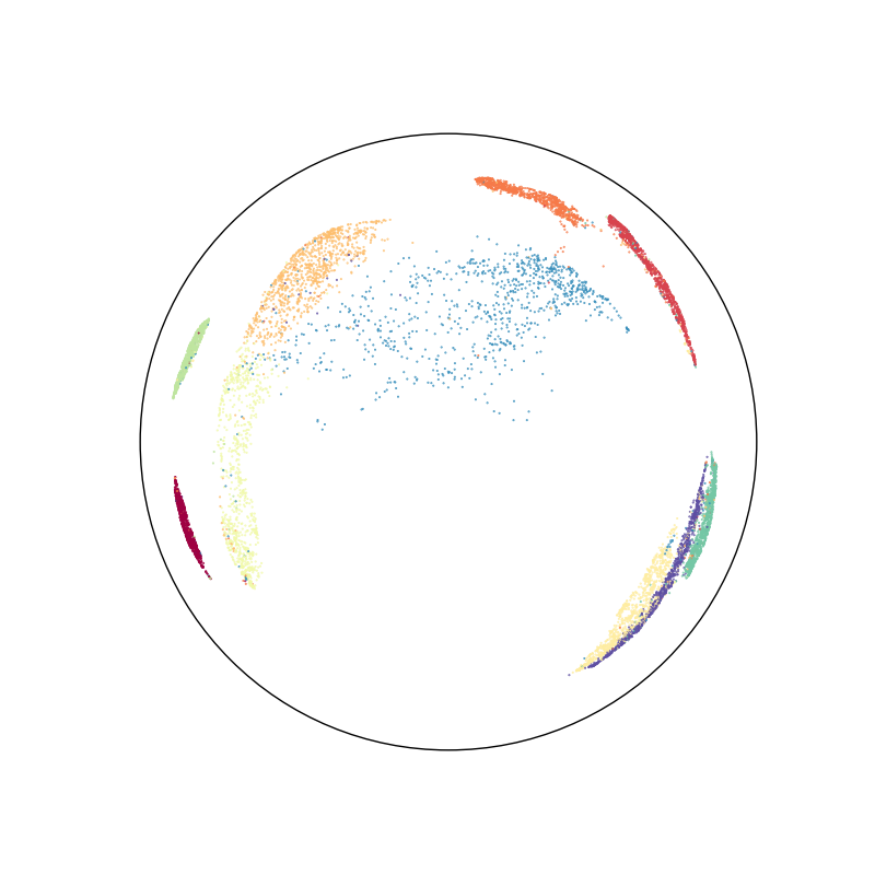
First of all, we use the umap algorithm to embed the MNIST dataset in the Poincare disk:
import torch

use_cuda = torch.cuda.is_available()
dtype = torch.cuda.FloatTensor if use_cuda else torch.FloatTensor

import numpy as np
import sklearn.datasets
import matplotlib.pyplot as plt
from mpl_toolkits.mplot3d import Axes3D
import umap

numpy = lambda x: x.cpu().numpy()


try:
    embedding = np.load("data/hyperbolic_embedding.npy")
    disk_x, disk_y = embedding[:, 0], embedding[:, 1]

    labels = np.load("data/hyperbolic_labels.npy")

except IOError:
    dataset = sklearn.datasets.fetch_openml("mnist_784")

    print(dataset.data.shape)

    features, labels = dataset.data, dataset.target.astype("int64")

    hyperbolic_mapper = umap.UMAP(target_metric="hyperboloid", random_state=42).fit(
        features
    )

    print("Hyperbolic embedding computed")

    x = hyperbolic_mapper.embedding_[:, 0]
    y = hyperbolic_mapper.embedding_[:, 1]
    z = np.sqrt(1 + np.sum(hyperbolic_mapper.embedding_**2, axis=1))

    disk_x = x / (1 + z)
    disk_y = y / (1 + z)
    embedding = np.stack((disk_x, disk_y)).T

    np.save("data/hyperbolic_embedding.npy", embedding)
    np.save("data/hyperbolic_labels.npy", labels)


fig = plt.figure(figsize=(8, 8))
ax = fig.add_subplot(111)
ax.scatter(disk_x, disk_y, c=labels, s=2000 / len(labels), cmap="Spectral")
boundary = plt.Circle((0, 0), 1, fc="none", ec="k")
ax.add_artist(boundary)
plt.axis("equal")
plt.axis([-1.1, 1.1, -1.1, 1.1])
ax.axis("off")
Out:
(-1.1, 1.1, -1.1, 1.1)
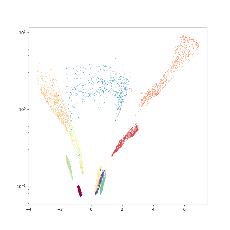
We then create a hyperbolic space of dimension 2, and visualize our embedding:
from monaco.hyperbolic import HyperbolicSpace, disk_to_halfplane

space = HyperbolicSpace(dimension=2, dtype=dtype)

X = torch.from_numpy(embedding).type(dtype)
X = disk_to_halfplane(X)

fig = plt.figure(figsize=(8, 8))

plt.scatter(numpy(X)[:, 0], numpy(X)[:, 1], c=labels, s=2000 / len(X), cmap="Spectral")
plt.yscale("log")


fig = plt.figure(figsize=(8, 8))
ax = fig.add_subplot(111)

space.scatter(X, "red")
space.draw_frame()
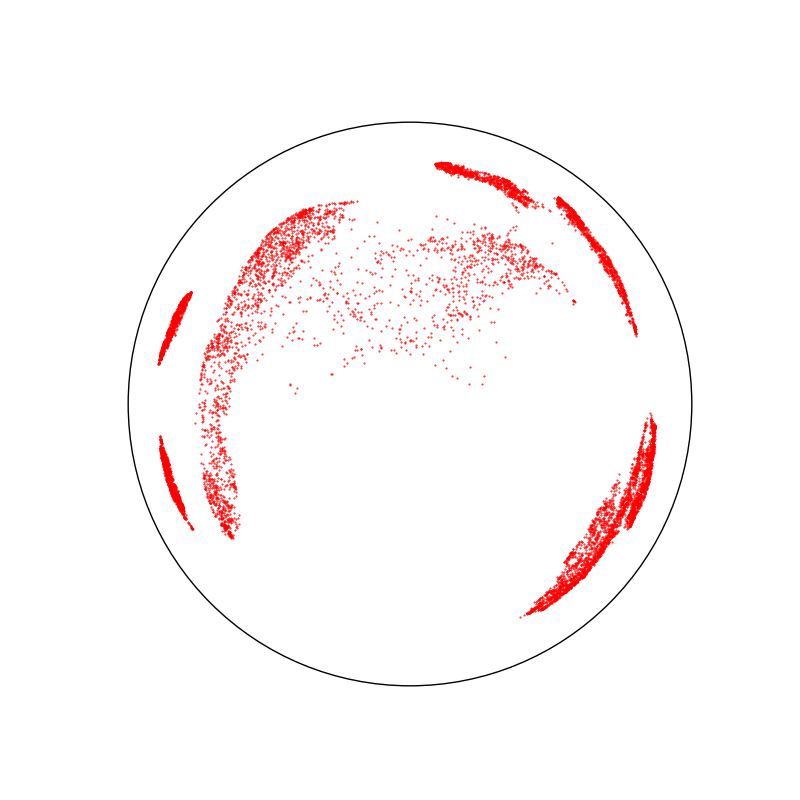
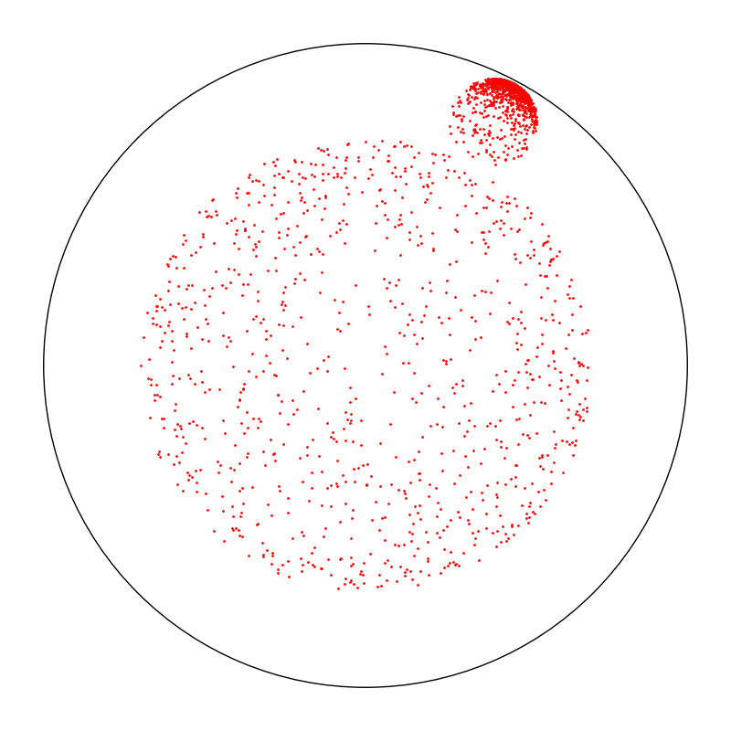
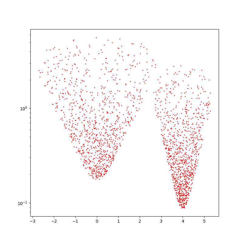
Under the hood, the Monaco package relies on the Poincare half-plane plane but displays all results in the Poincare disk. Here, we display two uniform samples in hyperbolic disks of radius 1.75.
from monaco.hyperbolic import BallProposal

proposal = BallProposal(space, scale=1.75)

A = torch.FloatTensor([0, 1]).type(dtype)
B = torch.FloatTensor([4, 0.5]).type(dtype)

ref = torch.stack((A,) * 1000 + (B,) * 1000, dim=0)

d_AB = 1 + ((A - B) ** 2).sum() / (2 * A[1] * B[1])
d_AB = (d_AB + (d_AB**2 - 1).sqrt()).log()
print(d_AB)


from monaco.hyperbolic import halfplane_to_disk

print(halfplane_to_disk(A))
C = halfplane_to_disk(B)
print(C)
R = (C**2).sum().sqrt()
d_IC = ((1 + R) / (1 - R)).log()
print(d_IC)


x = proposal.sample(ref)


# Display the initial configuration:
plt.figure(figsize=(8, 8))
space.scatter(x, "red")
space.draw_frame()
plt.tight_layout()


fig = plt.figure(figsize=(8, 8))
plt.scatter(numpy(x)[:, 0], numpy(x)[:, 1], c="red", s=2000 / len(x))
plt.yscale("log")
Out:
tensor(3.5401, device='cuda:0')
tensor([0., 0.], device='cuda:0')
tensor([0.4384, 0.8356], device='cuda:0')
tensor(3.5401, device='cuda:0')
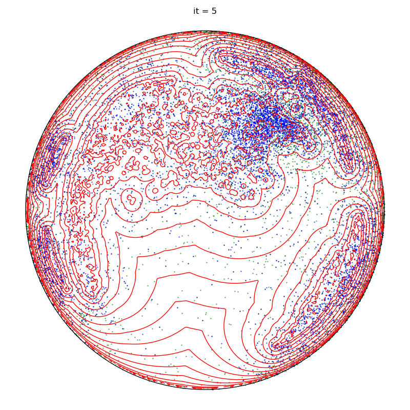
Monte Carlo sampling
We define an arbitrary potential in the hyperbolic plane: 10 times the square root of the distance to the nearest point in our MNIST embedding.
from pykeops.torch import LazyTensor


class DistanceDistribution(object):
    def __init__(self, points):
        self.points = points

    def potential(self, x):
        """Evaluates the potential on the point cloud x."""

        x_i = LazyTensor(x[:, None, :])
        y_j = LazyTensor(self.points[None, :, :])

        D_ij = ((x_i - y_j) ** 2).sum(-1)
        D_ij = 1 + D_ij / (2 * x_i[1] * y_j[1])
        D_ij = (D_ij + (D_ij**2 - 1).sqrt()).log()

        V_i = D_ij.min(dim=1)
        V_i = 10 * V_i.sqrt()
        return V_i.reshape(-1)  # (N,)


target = X if use_cuda else X[:100]

distribution = DistanceDistribution(target)
We then rely on the MOKA algorithm to generate samples efficiently.
from monaco.samplers import MOKA_CMC
N = 10000 if use_cuda else 50
start = 1.0 + torch.rand(N, 2).type(dtype)
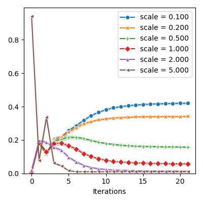
proposal = BallProposal(space, scale=[0.1, 0.2, 0.5, 1.0, 2.0, 5.0])
moka_sampler = MOKA_CMC(space, start, proposal, annealing=5).fit(distribution)
The code below generates some custom plots for our paper.
import numpy as np
import itertools
import torch

import seaborn as sns
from matplotlib import pyplot as plt

numpy = lambda x: x.cpu().numpy()

FIGSIZE = (4, 4)  # Small thumbnails for the paper
Out:
/home/.local/lib/python3.8/site-packages/seaborn/cm.py:1582: UserWarning: Trying to register the cmap 'rocket' which already exists.
  mpl_cm.register_cmap(_name, _cmap)
/home/.local/lib/python3.8/site-packages/seaborn/cm.py:1583: UserWarning: Trying to register the cmap 'rocket_r' which already exists.
  mpl_cm.register_cmap(_name + "_r", _cmap_r)
/home/.local/lib/python3.8/site-packages/seaborn/cm.py:1582: UserWarning: Trying to register the cmap 'mako' which already exists.
  mpl_cm.register_cmap(_name, _cmap)
/home/.local/lib/python3.8/site-packages/seaborn/cm.py:1583: UserWarning: Trying to register the cmap 'mako_r' which already exists.
  mpl_cm.register_cmap(_name + "_r", _cmap_r)
/home/.local/lib/python3.8/site-packages/seaborn/cm.py:1582: UserWarning: Trying to register the cmap 'icefire' which already exists.
  mpl_cm.register_cmap(_name, _cmap)
/home/.local/lib/python3.8/site-packages/seaborn/cm.py:1583: UserWarning: Trying to register the cmap 'icefire_r' which already exists.
  mpl_cm.register_cmap(_name + "_r", _cmap_r)
/home/.local/lib/python3.8/site-packages/seaborn/cm.py:1582: UserWarning: Trying to register the cmap 'vlag' which already exists.
  mpl_cm.register_cmap(_name, _cmap)
/home/.local/lib/python3.8/site-packages/seaborn/cm.py:1583: UserWarning: Trying to register the cmap 'vlag_r' which already exists.
  mpl_cm.register_cmap(_name + "_r", _cmap_r)
/home/.local/lib/python3.8/site-packages/seaborn/cm.py:1582: UserWarning: Trying to register the cmap 'flare' which already exists.
  mpl_cm.register_cmap(_name, _cmap)
/home/.local/lib/python3.8/site-packages/seaborn/cm.py:1583: UserWarning: Trying to register the cmap 'flare_r' which already exists.
  mpl_cm.register_cmap(_name + "_r", _cmap_r)
/home/.local/lib/python3.8/site-packages/seaborn/cm.py:1582: UserWarning: Trying to register the cmap 'crest' which already exists.
  mpl_cm.register_cmap(_name, _cmap)
/home/.local/lib/python3.8/site-packages/seaborn/cm.py:1583: UserWarning: Trying to register the cmap 'crest_r' which already exists.
  mpl_cm.register_cmap(_name + "_r", _cmap_r)
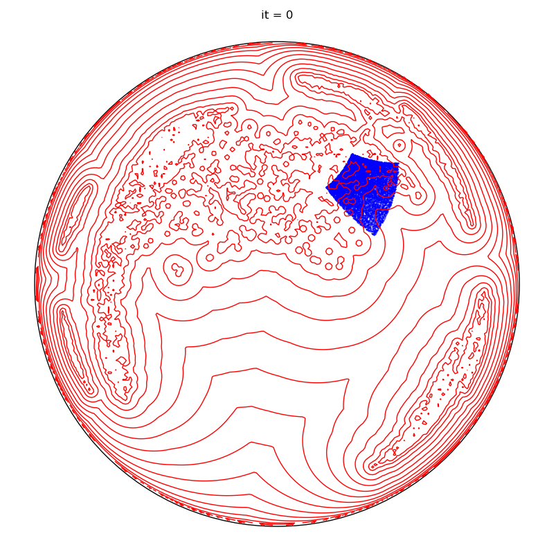
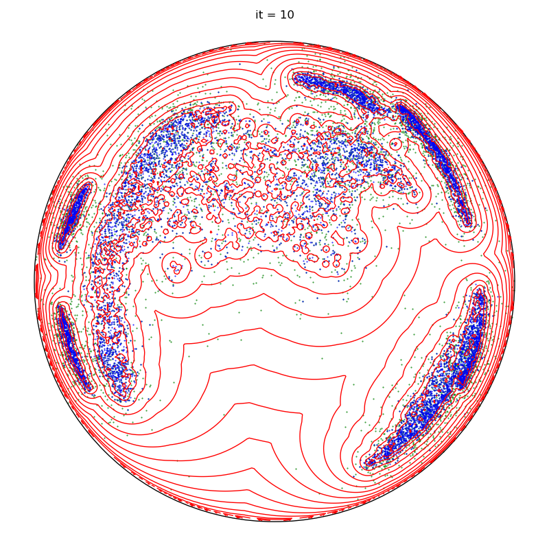
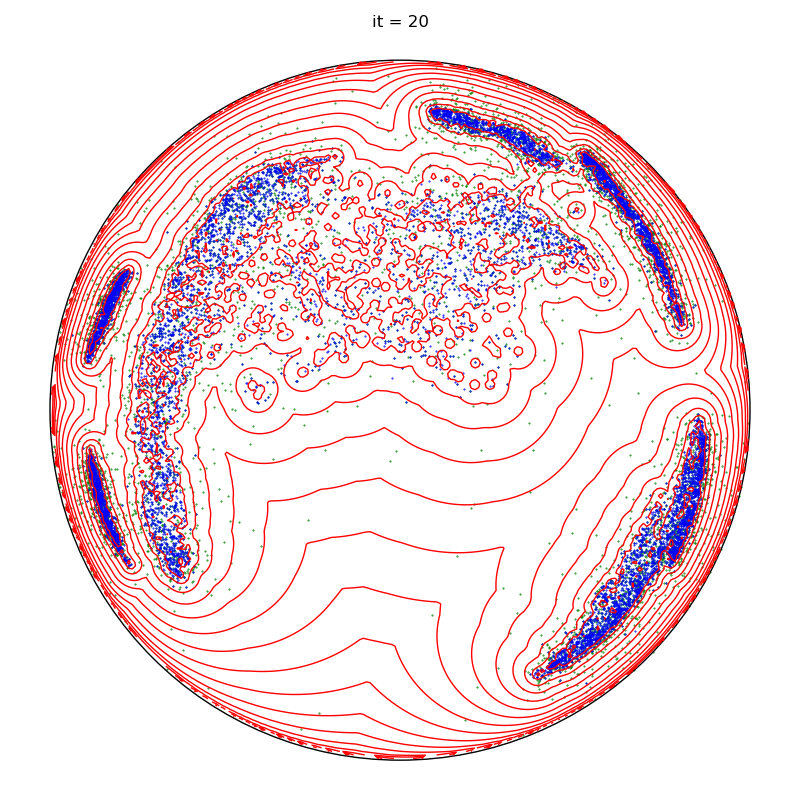
Fancy display of the current configuration:
def display(
    space,
    potential,
    sample,
    proposal_sample=None,
    proposal_potential=None,
    true_sample=None,
):

    if proposal_sample is not None:
        space.scatter(proposal_sample, "green")

    space.plot(potential, "red")
    space.scatter(sample, "blue")

    space.draw_frame()
Distances to the nearest neighbor:
def chamfer_distance(sou, tar):
    x_i = LazyTensor(sou[:, None, :])
    y_j = LazyTensor(tar[None, :, :])

    D_ij = ((x_i - y_j) ** 2).sum(-1)
    D_ij = 1 + D_ij / (2 * x_i[1] * y_j[1])
    D_ij = (D_ij + (D_ij**2 - 1).sqrt()).log()

    V_i = D_ij.min(dim=1)

    return V_i.mean().item()
Full results and statistics:
def display_samples(sampler, iterations=100, runs=5):
verbosity = sampler.verbose
sampler.verbose = True
start = sampler.x.clone()
iters, rates, errors, fluctuations, probas, constants = [], [], [], [], [], []
source_to_target, target_to_source = [], []
for run in range(runs):
x_prev = start.clone()
sampler.x[:] = start.clone()
sampler.iteration = 0
if run == runs - 1:
plt.figure(figsize=(8, 8))
display(sampler.space, sampler.distribution.potential, x_prev)
plt.title(f"it = 0")
plt.tight_layout()
to_plot = [1, 2, 5, 10, 20, 50, 100]
for it, info in enumerate(sampler):
x = info["sample"]
y = info.get("proposal", None)
u = info.get("log-weights", None)
source_to_target.append(chamfer_distance(x, target))
target_to_source.append(chamfer_distance(target, x))
iters.append(it)
try:
rates.append(info["rate"].item())
except KeyError:
None
try:
probas.append(info["probas"])
except KeyError:
None
try:
constants.append(info["normalizing constant"].item())
except KeyError:
None
try:
N = len(x)
errors.append(
sampler.space.discrepancy(x, sampler.distribution.sample(N)).item()
)
fluctuations.append(
sampler.space.discrepancy(
sampler.distribution.sample(N), sampler.distribution.sample(N)
).item()
)
except AttributeError:
None
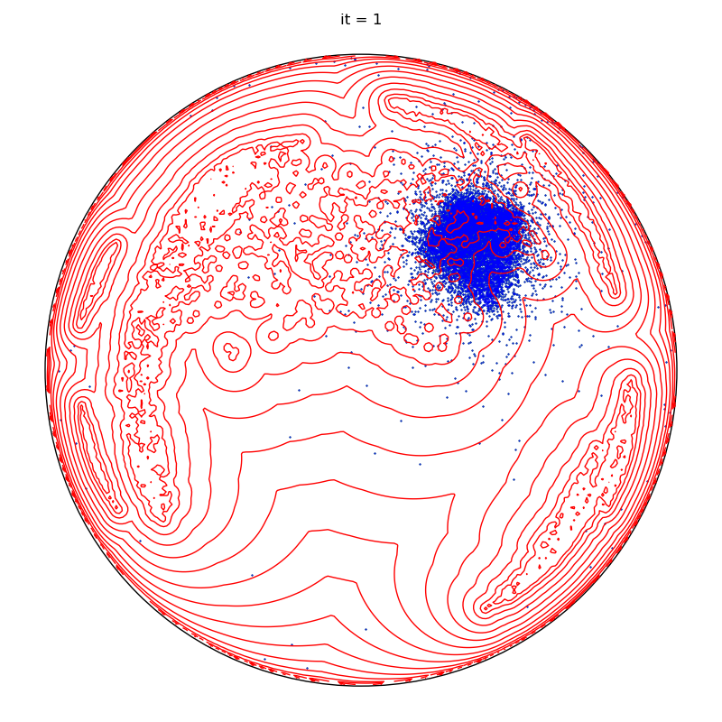
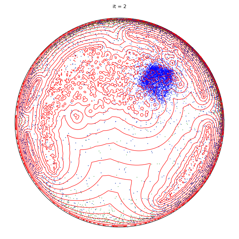
if run == runs - 1 and it + 1 in to_plot:
plt.figure(figsize=(8, 8))
try:
display(
sampler.space,
sampler.distribution.potential,
x,
y,
sampler.proposal.potential(x_prev, u),
sampler.distribution.sample(len(x)),
)
except AttributeError:
display(sampler.space, sampler.distribution.potential, x, y)
plt.title(f"it = {it+1}")
plt.tight_layout()
x_prev = x
if it > iterations:
break
iters = np.array(iters)
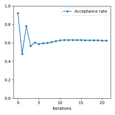
if rates != []:
rates = np.array(rates)
plt.figure(figsize=FIGSIZE)
sns.lineplot(
x=np.array(iters),
y=np.array(rates),
marker="o",
markersize=6,
label="Acceptance rate",
ci="sd",
)
plt.ylim(0, 1)
plt.xlabel("Iterations")
plt.tight_layout()
if errors != []:
errors = np.array(errors)
plt.figure(figsize=FIGSIZE)
sns.lineplot(
x=iters, y=errors, marker="o", markersize=6, label="Error", ci="sd"
)
if fluctuations != []:
fluctuations = np.array(fluctuations)
sns.lineplot(
x=iters,
y=fluctuations,
marker="X",
markersize=6,
label="Fluctuations",
ci="sd",
)
plt.xlabel("Iterations")
plt.ylim(bottom=0.0)
plt.tight_layout()
if probas != []:
probas = numpy(torch.stack(probas)).T
plt.figure(figsize=FIGSIZE)
markers = itertools.cycle(("o", "X", "P", "D", "^", "<", "v", ">", "*"))
for scale, proba, marker in zip(sampler.proposal.s, probas, markers):
sns.lineplot(
x=iters,
y=proba,
marker=marker,
markersize=6,
label="scale = {:.3f}".format(scale),
ci="sd",
)
plt.xlabel("Iterations")
plt.ylim(bottom=0.0)
plt.tight_layout()
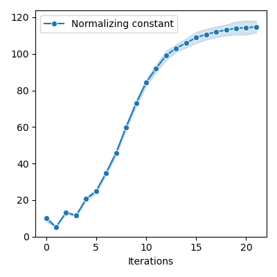
if constants != []:
plt.figure(figsize=FIGSIZE)
constants = np.array(constants)
sns.lineplot(
x=iters,
y=constants,
marker="o",
markersize=6,
label="Normalizing constant",
ci="sd",
)
plt.xlabel("Iterations")
plt.ylim(bottom=0.0)
plt.tight_layout()
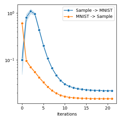
source_to_target = np.array(source_to_target)
target_to_source = np.array(target_to_source)
plt.figure(figsize=FIGSIZE)
sns.lineplot(
x=iters,
y=source_to_target,
marker="o",
markersize=6,
label="Sample -> MNIST",
ci="sd",
)
sns.lineplot(
x=iters,
y=target_to_source,
marker="o",
markersize=6,
label="MNIST -> Sample",
ci="sd",
)
plt.xlabel("Iterations")
# plt.ylim(bottom = 0.)
plt.yscale("log")
plt.tight_layout()
sampler.verbose = verbosity
to_return = {
"iteration": iters,
"rate": rates,
"normalizing constant": constants,
"error": errors,
"fluctuation": fluctuations,
"probas": probas,
"source_to_target": source_to_target,
"target_to_source": target_to_source,
}
return to_return
We’re good to go!
info = display_samples(moka_sampler, iterations=20, runs=50)

plt.show()
Total running time of the script: ( 0 minutes 18.534 seconds)