Note
Click here to download the full example code
Sampling on a banana distribution
We discuss the performances of several Monte Carlo samplers on a toy 2D example.
Introduction
First of all, some standard imports.
import numpy as np
import torch
from matplotlib import pyplot as plt
import sys

sys.setrecursionlimit(10000)
# plt.rcParams.update({"figure.max_open_warning": 0})

use_cuda = torch.cuda.is_available()
dtype = torch.cuda.FloatTensor if use_cuda else torch.FloatTensor
Our sampling space:
from monaco.euclidean import EuclideanSpace

D = 2
space = EuclideanSpace(dimension=D, dtype=dtype)
Our toy target distribution:
from monaco.euclidean import GaussianMixture, UnitPotential

N, M = (10000 if use_cuda else 50), 5
nruns = 50
niter = 80


test_case = "gaussians"

if test_case == "gaussians":
    # Let's generate a blend of peaky Gaussians, in the unit square:
    m = torch.tensor([[0.2, 0.8], [0.8, 0.8], [0.5, 0.1]]).type(dtype)  # mean
    s = torch.tensor([0.02, 0.02, 0.02]).type(dtype)  # deviation
    w = torch.tensor([0.3, 0.3, 0.4]).type(dtype)  # weights
    w = w**2

    w = w / w.sum()  # normalize weights

    distribution_gauss = GaussianMixture(space, m, s, w)


from monaco.euclidean import GaussianMixture, UnitPotential
from torch.distributions.multivariate_normal import MultivariateNormal


space = EuclideanSpace(dimension=D, dtype=dtype)


def sinc_potential(x, stripes=3):
    sqnorm = (x**2).sum(-1)
    V_i = np.pi * stripes * sqnorm
    V_i = (V_i.sin() / V_i) ** 2
    return -V_i.log()


def banana_log_pdf(x):
    b = 0.03
    y = x.clone().detach()
    y[:, 1] = y[:, 1] + b * y[:, 0] ** 2 - 100.0 * b
    return -0.5 * (y[:, 0] ** 2 / 100.0 + y[:, 1] ** 2) - 4.1404621594


def banana_potential_plus(x):
    # Add a constant for the rejection sampling
    return -banana_log_pdf(100 * (x - 0.5)) - 9.21034037198


distribution_banana = UnitPotential(space, banana_potential_plus)

alpha = torch.tensor(0.5).type(dtype)


def mix_potential_plus(x):
    # Add a constant for the rejection
    A = -banana_potential_plus(x) + alpha.log()
    B = -distribution_gauss.potential(x) + (1 - alpha).log()
    AB = torch.cat((A[:, None], B[:, None]), dim=1)
    C = AB.logsumexp(dim=1)
    return -C + 5 - 0.46  # Minimum on the unit square ~ 0


distribution = UnitPotential(space, mix_potential_plus)
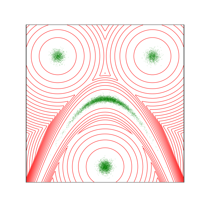
Display the target density, with a typical sample.
plt.figure(figsize=(8, 8))
space.scatter(distribution.sample(N), "green")
space.plot(distribution.potential, "red")
space.draw_frame()
As an error criterion, we use the Energy Distance:
if False:
    from monaco.euclidean import squared_distances

    EDtest = np.zeros(101)
    for i in range(100):
        perfect_sample_2 = distribution.sample(N)
        perfect_sample = distribution.sample(N)
        n, m = len(perfect_sample), len(perfect_sample_2)
        D_xx = squared_distances(perfect_sample, perfect_sample).sqrt().sum(dim=1).sum()
        D_xy = (
            squared_distances(perfect_sample, perfect_sample_2).sqrt().sum(dim=1).sum()
        )
        D_yy = (
            squared_distances(perfect_sample_2, perfect_sample_2)
            .sqrt()
            .sum(dim=1)
            .sum()
        )
        EDtest[i] = D_xy / (n * m) - 0.5 * (D_xx / (n * n) + D_yy / (m * m))

    print(EDtest[range(100)])
    print(np.mean(EDtest[range(100)]))
    print(np.std(EDtest[range(100)]))
Sampling
perfect_sample = distribution.sample(N)


def perfect_sampling(*args, **kwargs):
    return perfect_sample


distribution.sample = perfect_sampling


def mix_potential0(x):
    A = -banana_potential_plus(x) + alpha.log()
    B = -distribution_gauss.potential(x) + (1 - alpha).log()
    AB = torch.cat((A[:, None], B[:, None]), dim=1)
    C = AB.logsumexp(dim=1)
    return -C


distribution.potential = mix_potential0
We start from a very poor initialization, thus simulating the challenge of sampling an unknown distribution.
start = 0.9 + 0.1 * torch.rand(N, D).type(dtype) # start in a corner
For exploration, we generate a fraction of our samples using a simple uniform distribution.
from monaco.euclidean import UniformProposal
from monaco.euclidean import GaussianProposal

exploration = 0.01
exploration_proposal = GaussianProposal(space, scale=0.3)
annealing = None

scale = 0.01
multi_scale = [0.01, 0.03, 0.1, 0.3]
Our proposal will stay the same throughout the experiments: a combination of uniform samples on balls with radii that range from 1/1000 to 0.3.
from monaco.euclidean import BallProposal

proposal = BallProposal(
    space,
    scale=scale,
    exploration=exploration,
    exploration_proposal=exploration_proposal,
)
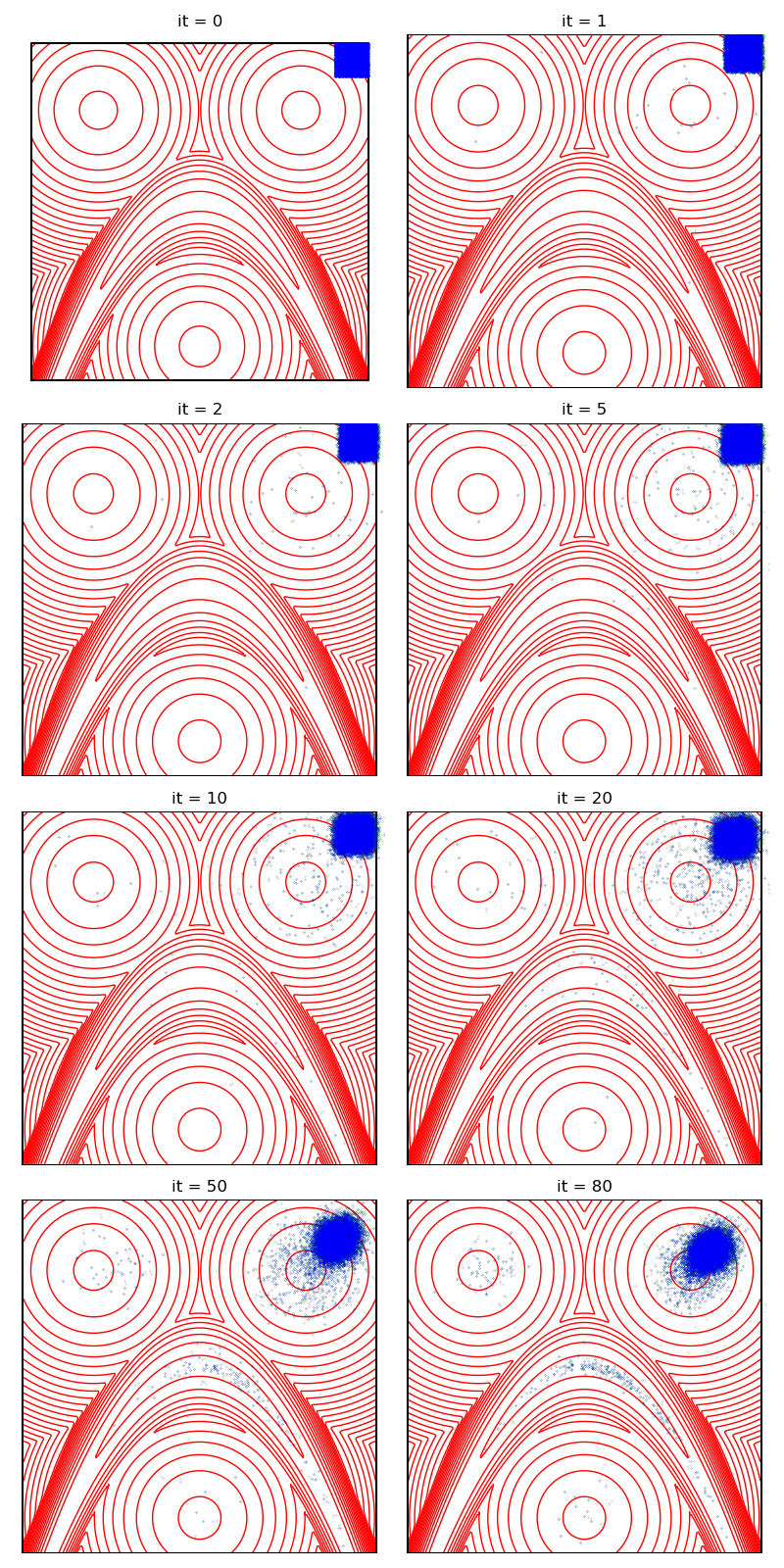
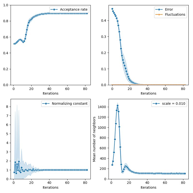
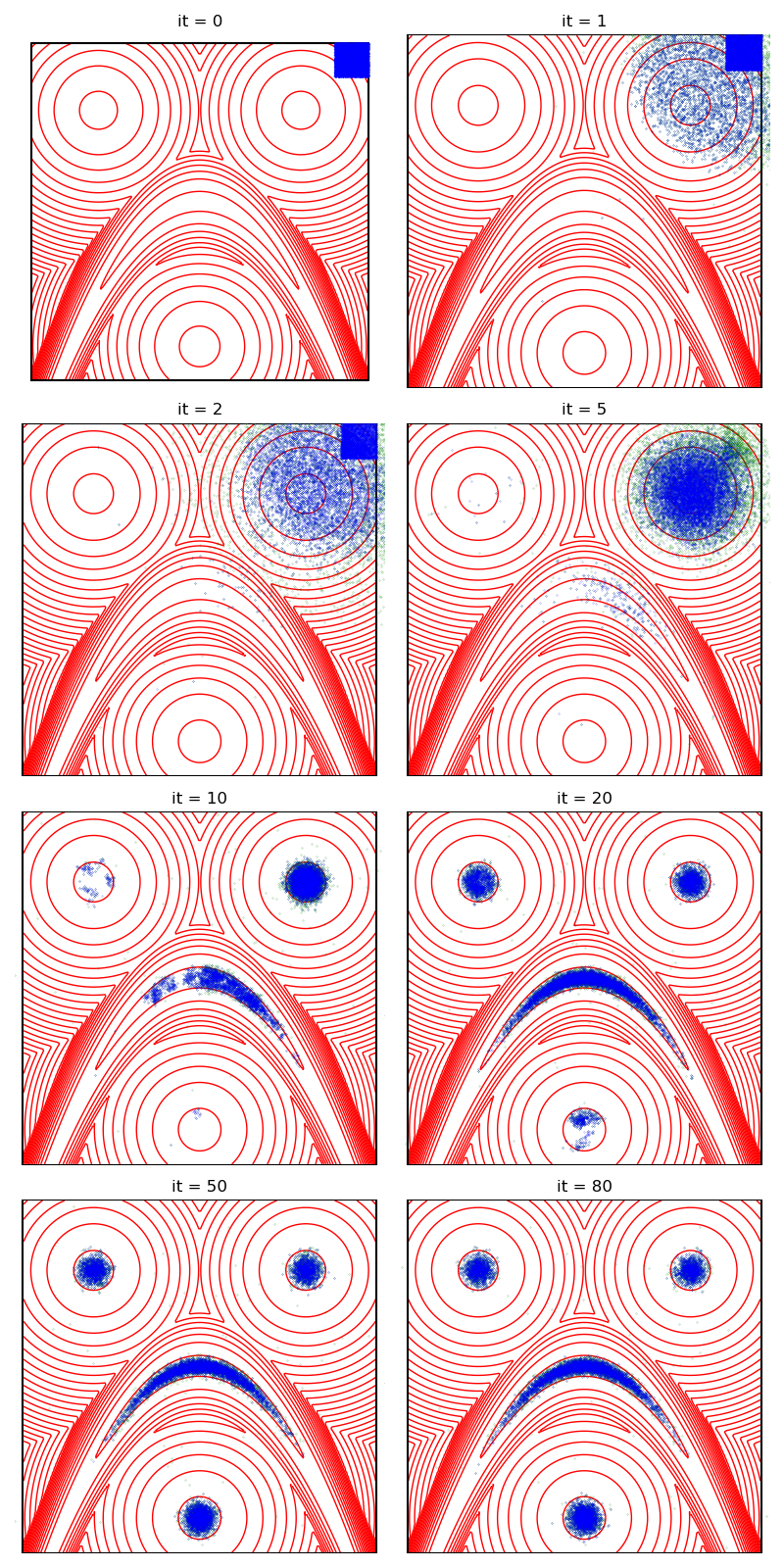
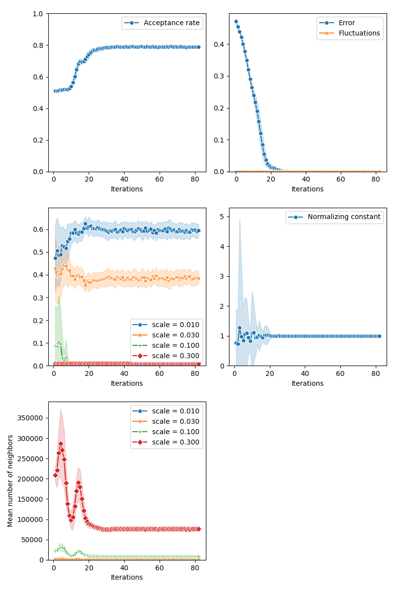
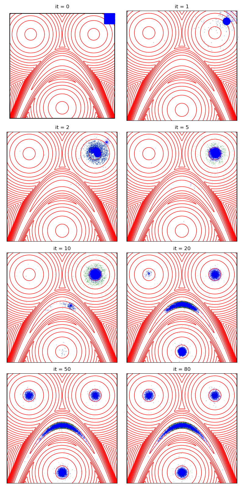
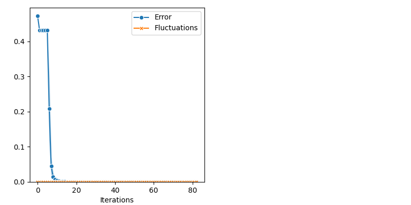
First of all, we illustrate a run of the standard Metropolis-Hastings algorithm, parallelized on the GPU:
from monaco.samplers import display_samples

info = {}

from monaco.samplers import ParallelMetropolisHastings

pmh_sampler = ParallelMetropolisHastings(
    space, start, proposal, annealing=annealing
).fit(distribution)
info["PMH"] = display_samples(pmh_sampler, iterations=niter, runs=nruns)
Out:
/home/.local/lib/python3.8/site-packages/seaborn/cm.py:1582: UserWarning: Trying to register the cmap 'rocket' which already exists.
  mpl_cm.register_cmap(_name, _cmap)
/home/.local/lib/python3.8/site-packages/seaborn/cm.py:1583: UserWarning: Trying to register the cmap 'rocket_r' which already exists.
  mpl_cm.register_cmap(_name + "_r", _cmap_r)
/home/.local/lib/python3.8/site-packages/seaborn/cm.py:1582: UserWarning: Trying to register the cmap 'mako' which already exists.
  mpl_cm.register_cmap(_name, _cmap)
/home/.local/lib/python3.8/site-packages/seaborn/cm.py:1583: UserWarning: Trying to register the cmap 'mako_r' which already exists.
  mpl_cm.register_cmap(_name + "_r", _cmap_r)
/home/.local/lib/python3.8/site-packages/seaborn/cm.py:1582: UserWarning: Trying to register the cmap 'icefire' which already exists.
  mpl_cm.register_cmap(_name, _cmap)
/home/.local/lib/python3.8/site-packages/seaborn/cm.py:1583: UserWarning: Trying to register the cmap 'icefire_r' which already exists.
  mpl_cm.register_cmap(_name + "_r", _cmap_r)
/home/.local/lib/python3.8/site-packages/seaborn/cm.py:1582: UserWarning: Trying to register the cmap 'vlag' which already exists.
  mpl_cm.register_cmap(_name, _cmap)
/home/.local/lib/python3.8/site-packages/seaborn/cm.py:1583: UserWarning: Trying to register the cmap 'vlag_r' which already exists.
  mpl_cm.register_cmap(_name + "_r", _cmap_r)
/home/.local/lib/python3.8/site-packages/seaborn/cm.py:1582: UserWarning: Trying to register the cmap 'flare' which already exists.
  mpl_cm.register_cmap(_name, _cmap)
/home/.local/lib/python3.8/site-packages/seaborn/cm.py:1583: UserWarning: Trying to register the cmap 'flare_r' which already exists.
  mpl_cm.register_cmap(_name + "_r", _cmap_r)
/home/.local/lib/python3.8/site-packages/seaborn/cm.py:1582: UserWarning: Trying to register the cmap 'crest' which already exists.
  mpl_cm.register_cmap(_name, _cmap)
/home/.local/lib/python3.8/site-packages/seaborn/cm.py:1583: UserWarning: Trying to register the cmap 'crest_r' which already exists.
  mpl_cm.register_cmap(_name + "_r", _cmap_r)
Then, the standard Collective Monte Carlo method:
from monaco.samplers import CMC

proposal = BallProposal(
    space,
    scale=scale,
    exploration=exploration,
    exploration_proposal=exploration_proposal,
)

cmc_sampler = CMC(space, start, proposal, annealing=None).fit(distribution)
info["CMC"] = display_samples(cmc_sampler, iterations=niter, runs=nruns)
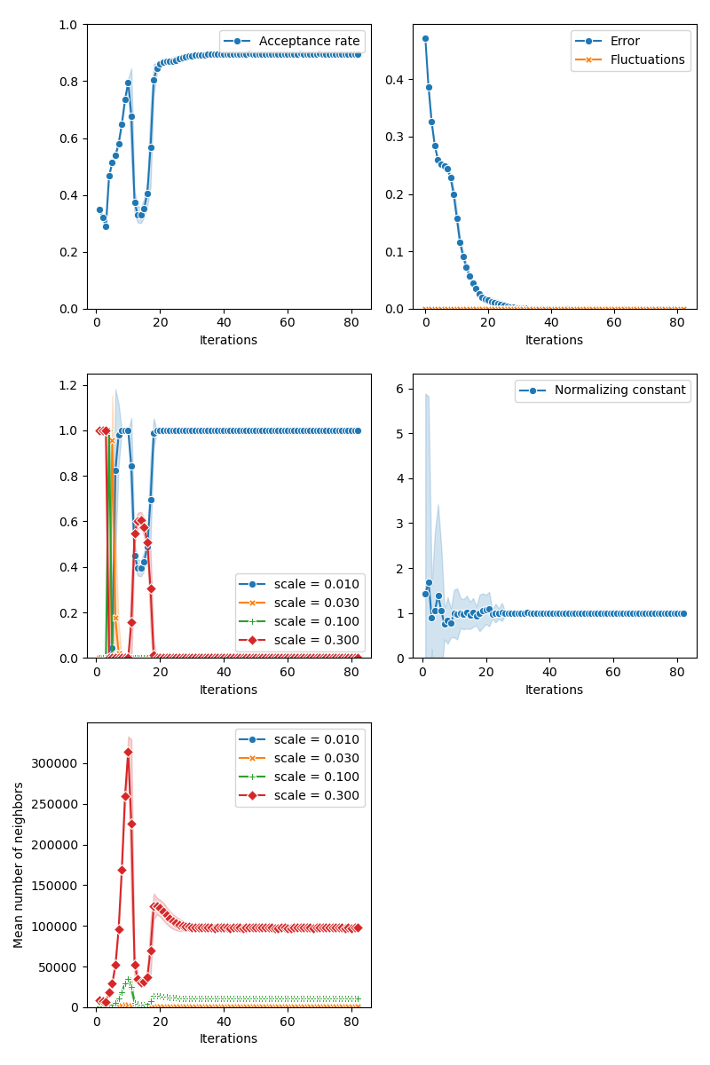
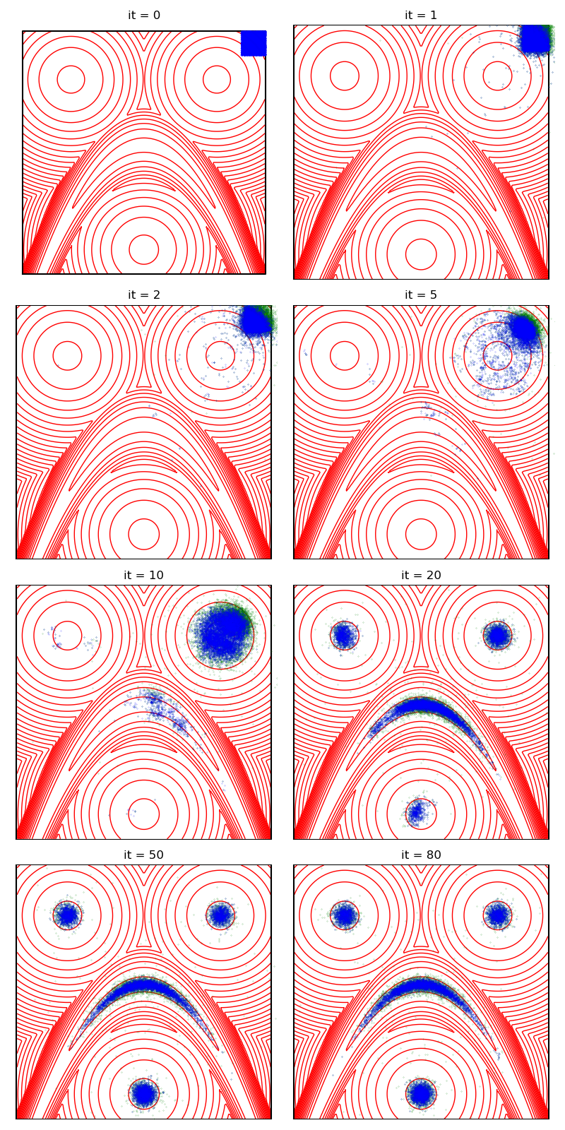
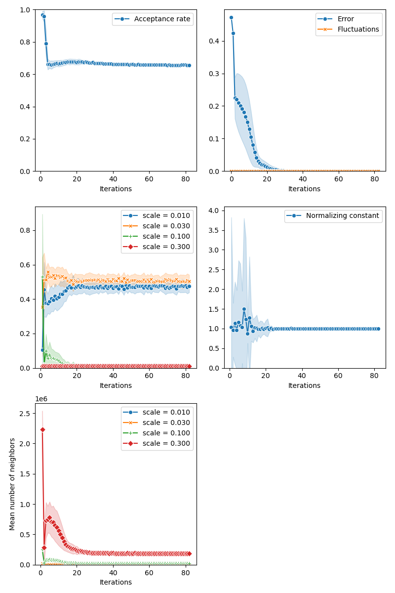
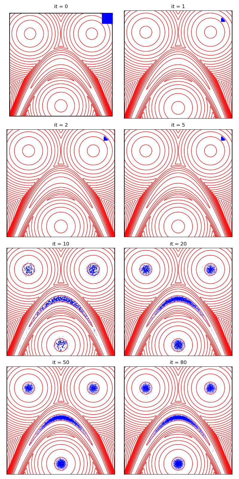
With a Markovian selection of the kernel bandwidth:
from monaco.samplers import MOKA_Markov_CMC

proposal = BallProposal(
    space,
    scale=multi_scale,
    exploration=exploration,
    exploration_proposal=exploration_proposal,
)

moka_markov_sampler = MOKA_Markov_CMC(space, start, proposal, annealing=annealing).fit(
    distribution
)
info["MOKA Markov"] = display_samples(moka_markov_sampler, iterations=niter, runs=nruns)
And a non-Markovian selection of the kernel bandwidth:
from monaco.samplers import MOKA_CMC

proposal = BallProposal(
    space,
    scale=multi_scale,
    exploration=exploration,
    exploration_proposal=exploration_proposal,
)

moka_sampler = MOKA_CMC(space, start, proposal, annealing=annealing).fit(distribution)
info["MOKA"] = display_samples(moka_sampler, iterations=niter, runs=nruns)
CMC with Richardson-Lucy deconvolution:
from monaco.samplers import MOKA_KIDS_CMC

proposal = BallProposal(
    space,
    scale=multi_scale,
    exploration=exploration,
    exploration_proposal=exploration_proposal,
)

moka_kids_sampler = MOKA_KIDS_CMC(
    space, start, proposal, annealing=annealing, iterations=50
).fit(distribution)
info["MOKA_KIDS"] = display_samples(moka_kids_sampler, iterations=niter, runs=nruns)
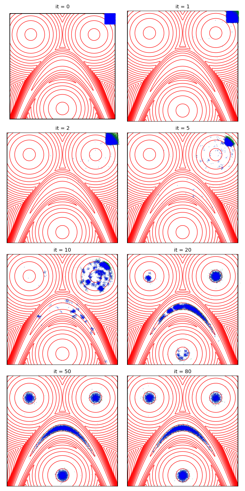
Finally, the Non Parametric Adaptive Importance Sampler, an efficient non-Markovian method with an extensive memory usage:
from monaco.samplers import SAIS

proposal = BallProposal(
    space,
    scale=scale,
    exploration=exploration,
    exploration_proposal=exploration_proposal,
)


class Q_0(object):
    def __init__(self):
        None

    def sample(self, n):
        return 0.9 + 0.1 * torch.rand(n, D).type(dtype)

    def potential(self, x):
        v = 100000 * torch.ones(len(x), 1).type_as(x)
        v[(x - 0.95).abs().max(1)[0] < 0.05] = -np.log(1 / 0.1)
        return v.view(-1)


q0 = Q_0()

sais_sampler = SAIS(
    space, start, proposal, annealing=True, scale0=0.5, q0=q0, N=N, sample_size=N, T0=10
).fit(distribution)
info["SAIS"] = display_samples(sais_sampler, iterations=niter, runs=nruns)
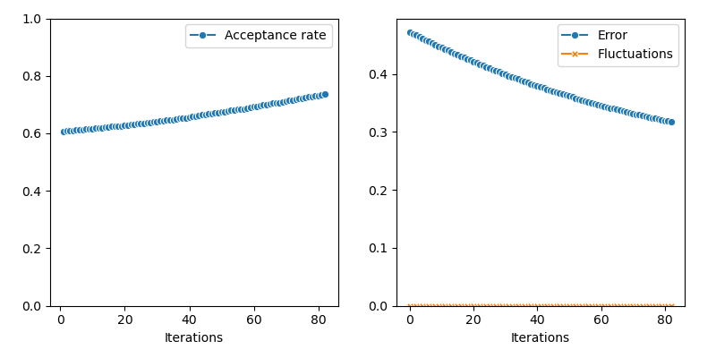
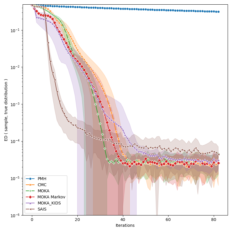
Comparative benchmark:
import itertools
import seaborn as sns

iters = info["PMH"]["iteration"]


def display_line(key, marker):
    sns.lineplot(
        x=info[key]["iteration"],
        y=info[key]["error"],
        label=key,
        marker=marker,
        markersize=6,
        ci="sd",
    )


plt.figure(figsize=(8, 8))
markers = itertools.cycle(("o", "X", "P", "D", "^", "<", "v", ">", "*"))

# for key, marker in zip(["PMH", "CMC","MOKA", "MOKA Markov", "KIDS", "MOKA_KIDS", "SAIS"], markers):
for key, marker in zip(
    ["PMH", "CMC", "MOKA", "MOKA Markov", "MOKA_KIDS", "SAIS"], markers
):
    display_line(key, marker)


plt.xlabel("Iterations")
plt.ylabel("ED ( sample, true distribution )")
plt.ylim(bottom=1e-6)
plt.yscale("log")

plt.tight_layout()


plt.show()
Total running time of the script: ( 26 minutes 37.715 seconds)