Sampling in 1D

We discuss the performances of several Monte Carlo samplers on a toy 1D example.

Introduction

First of all, some standard imports.

import numpy as np
import torch
from matplotlib import pyplot as plt

plt.rcParams.update({"figure.max_open_warning": 0})

use_cuda = torch.cuda.is_available()
dtype = torch.cuda.FloatTensor if use_cuda else torch.FloatTensor

Our sampling space:

from monaco.euclidean import EuclideanSpace

D = 1
space = EuclideanSpace(dimension=D, dtype=dtype)

Our toy target distribution:

from monaco.euclidean import GaussianMixture, UnitPotential

N, M = (10000 if use_cuda else 50), 5
Nlucky = 100 if use_cuda else 2
nruns = 5

test_case = "sophia"

if test_case == "gaussians":
    # Let's generate a blend of peaky Gaussians, in the unit square:
    m = torch.rand(M, D).type(dtype)  # mean
    s = torch.rand(M).type(dtype)  # deviation
    w = torch.rand(M).type(dtype)  # weights

    m = 0.25 + 0.5 * m
    s = 0.005 + 0.1 * (s**6)
    w = w / w.sum()  # normalize weights

    distribution = GaussianMixture(space, m, s, w)


elif test_case == "sophia":
    m = torch.FloatTensor([0.5, 0.1, 0.2, 0.8, 0.9]).type(dtype)[:, None]
    s = torch.FloatTensor([0.15, 0.005, 0.002, 0.002, 0.005]).type(dtype)
    w = torch.FloatTensor([0.1, 2 / 12, 1 / 12, 1 / 12, 2 / 12]).type(dtype)
    w = w / w.sum()  # normalize weights

    distribution = GaussianMixture(space, m, s, w)


elif test_case == "ackley":

    def ackley_potential(x, stripes=15):
        f_1 = 20 * (-0.2 * (((x - 0.5) * stripes) ** 2).mean(-1).sqrt()).exp()
        f_2 = ((2 * np.pi * ((x - 0.5) * stripes)).cos().mean(-1)).exp()

        return -(f_1 + f_2 - np.exp(1) - 20) / stripes

    distribution = UnitPotential(space, ackley_potential)

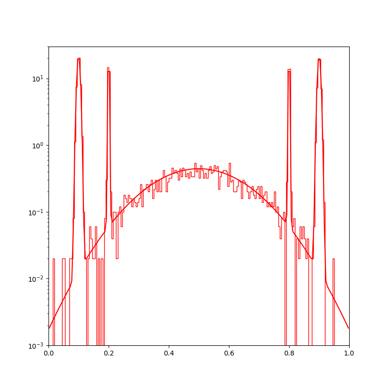
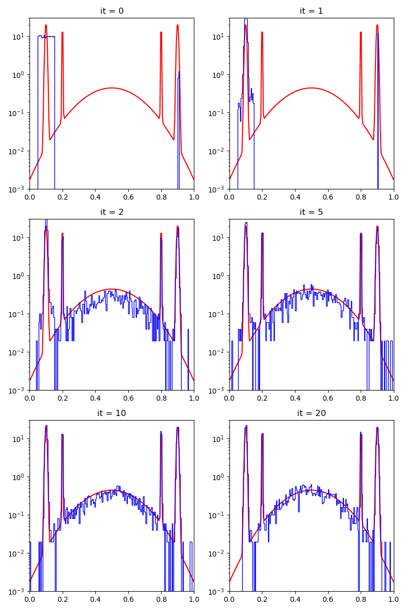
Display the target density, with a typical sample.

plt.figure(figsize=(8, 8))
space.scatter(distribution.sample(N), "red")
space.plot(distribution.potential, "red")
space.draw_frame()

Sampling

We start from a relatively bad start, albeit with 1 / 100 of lucky samples on of the modes of the target distribution.

start = 0.05 + 0.1 * torch.rand(N, D).type(dtype)
start[:Nlucky] = 0.9 + 0.01 * torch.rand(Nlucky, D).type(dtype)

For exploration, we generate a fraction of our samples using a simple uniform distribution.

from monaco.euclidean import UniformProposal

exploration = 0.05
exploration_proposal = UniformProposal(space)

Our proposal will stay the same throughout the experiments: a combination of uniform samples on balls with radii that range from 1/1000 to 0.3.

from monaco.euclidean import BallProposal

proposal = BallProposal(
    space,
    scale=[0.001, 0.003, 0.01, 0.03, 0.1, 0.3],
    exploration=exploration,
    exploration_proposal=exploration_proposal,
)

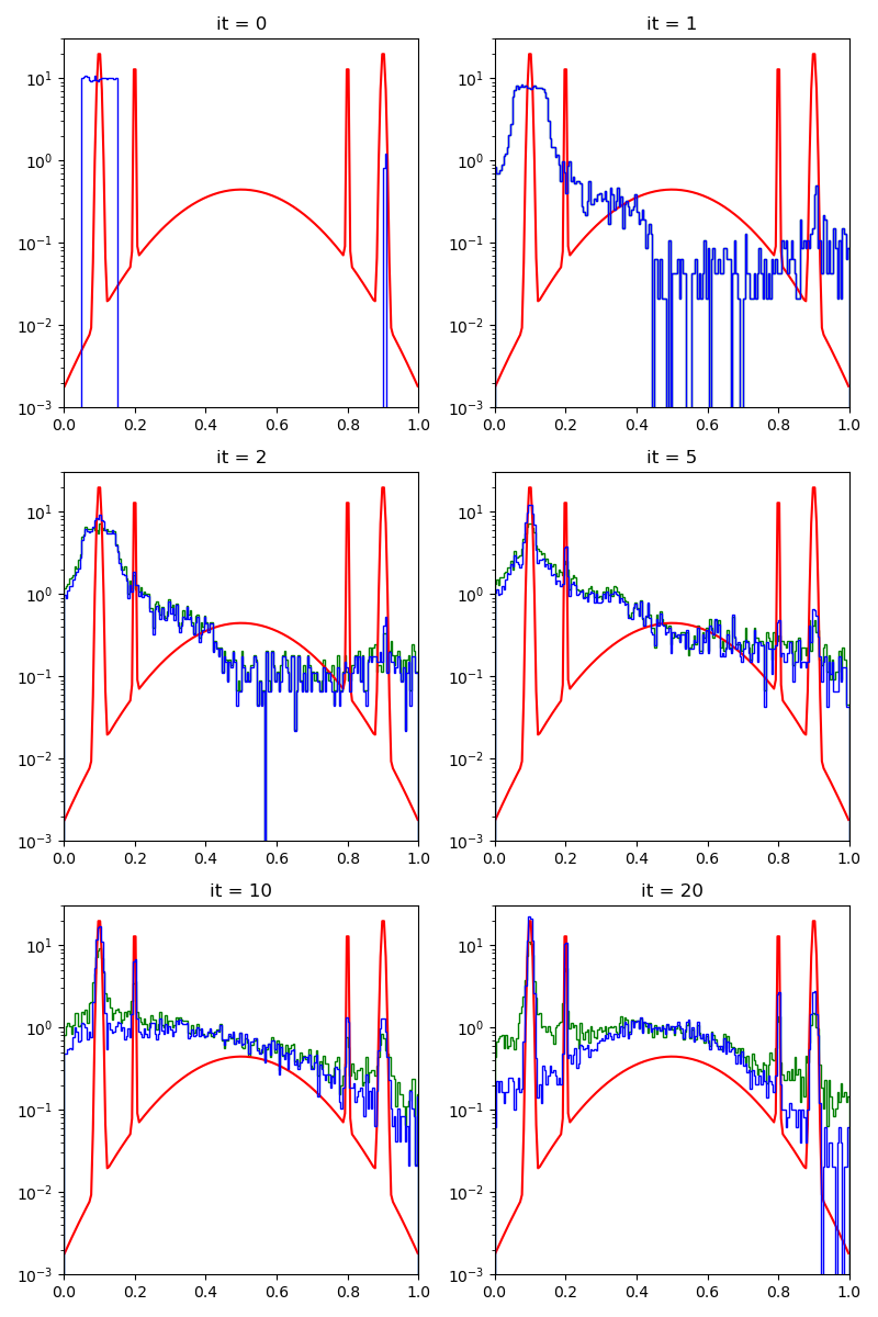
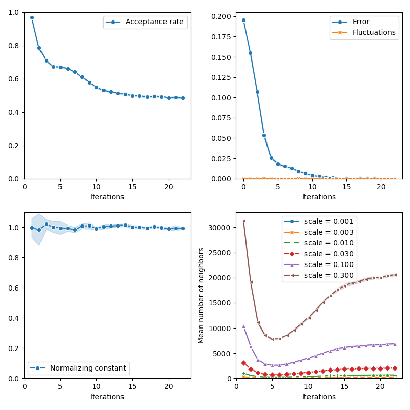
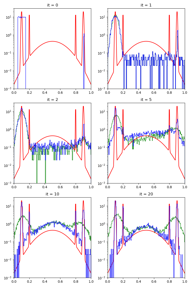
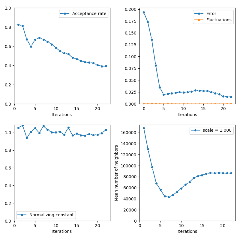
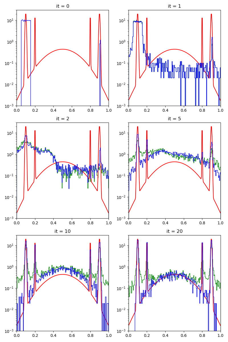
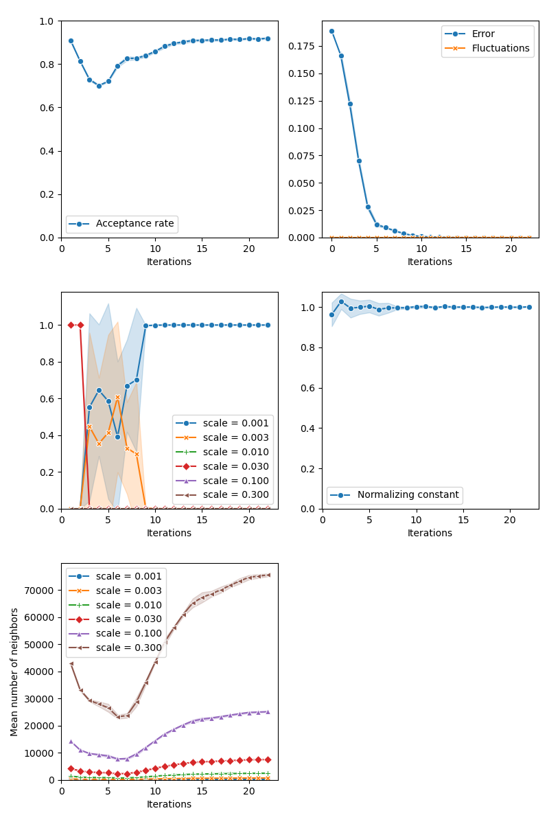
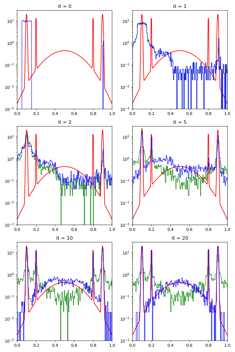
First of all, we illustrate a run of the standard Metropolis-Hastings algorithm, parallelized on the GPU:

info = {}

from monaco.samplers import ParallelMetropolisHastings, display_samples

pmh_sampler = ParallelMetropolisHastings(space, start, proposal, annealing=5).fit(
    distribution
)
info["PMH"] = display_samples(pmh_sampler, iterations=20, runs=nruns)

• 
• 

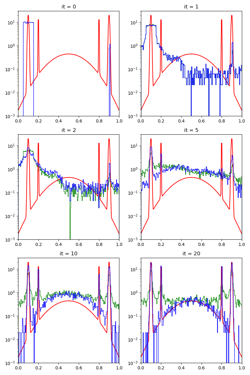
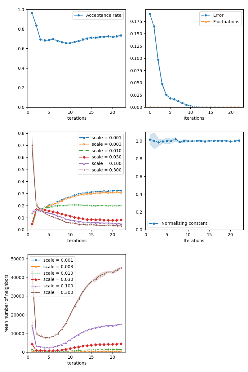
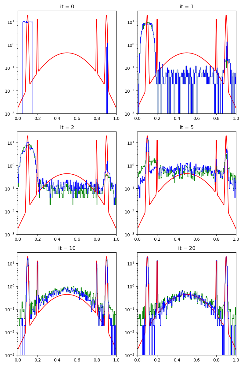
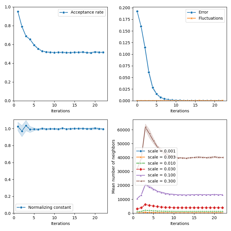
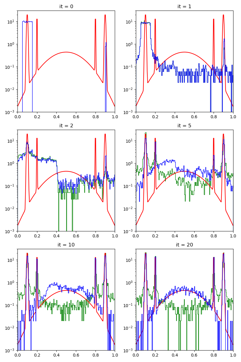
Then, the standard Collective Monte Carlo method:

from monaco.samplers import CMC

cmc_sampler = CMC(space, start, proposal, annealing=5).fit(distribution)
info["CMC"] = display_samples(cmc_sampler, iterations=20, runs=nruns)

• 
• 

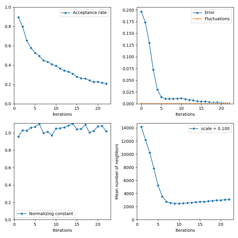
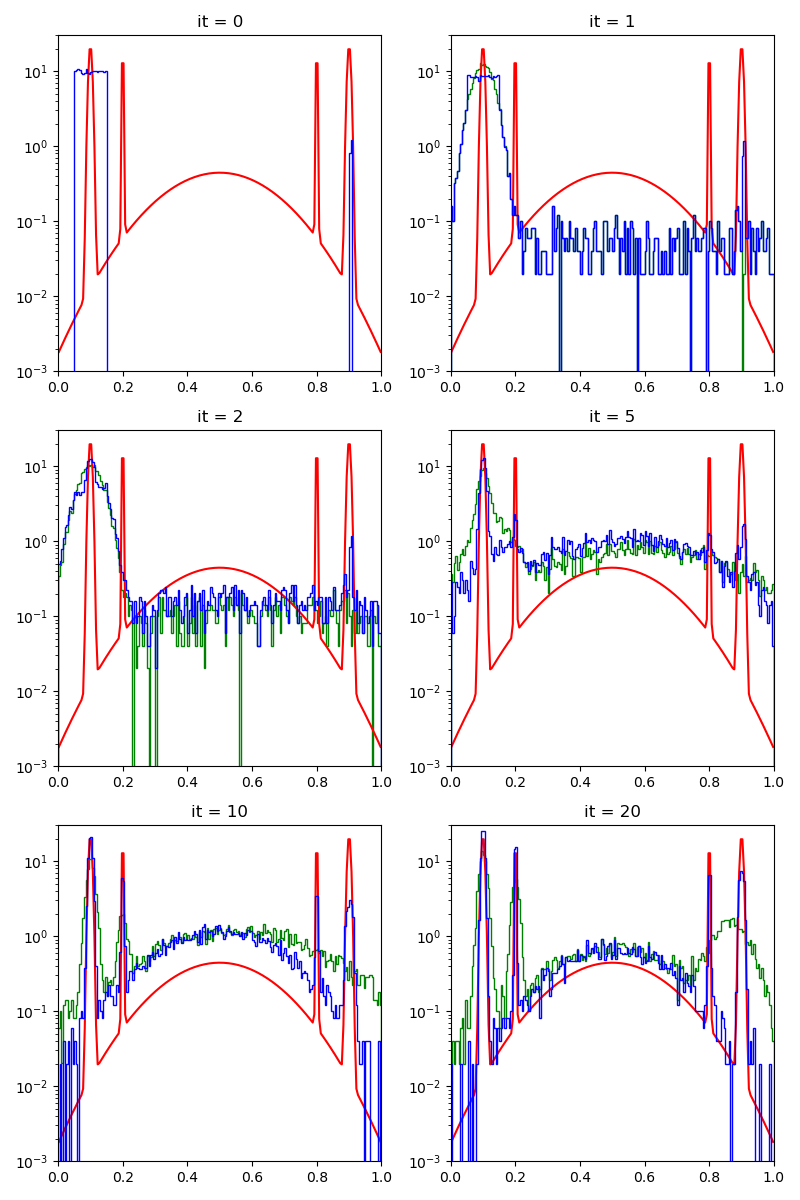
BGK - Collective Monte Carlo method:

from monaco.samplers import Ada_CMC
from monaco.euclidean import GaussianProposal

gaussian_proposal = GaussianProposal(
    space,
    scale=[0.1],
    exploration=exploration,
    exploration_proposal=exploration_proposal,
)

bgk_sampler = Ada_CMC(space, start, gaussian_proposal, annealing=5).fit(distribution)
info["BGK_CMC"] = display_samples(bgk_sampler, iterations=20, runs=1)

• 
• 

GMM - Collective Monte Carlo method:

from monaco.euclidean import GMMProposal

gmm_proposal = GMMProposal(
    space,
    n_classes=100,
    exploration=exploration,
    exploration_proposal=exploration_proposal,
)

gmm_sampler = Ada_CMC(space, start, gmm_proposal, annealing=5).fit(distribution)
info["GMM_CMC"] = display_samples(gmm_sampler, iterations=20, runs=1)

• 
• 

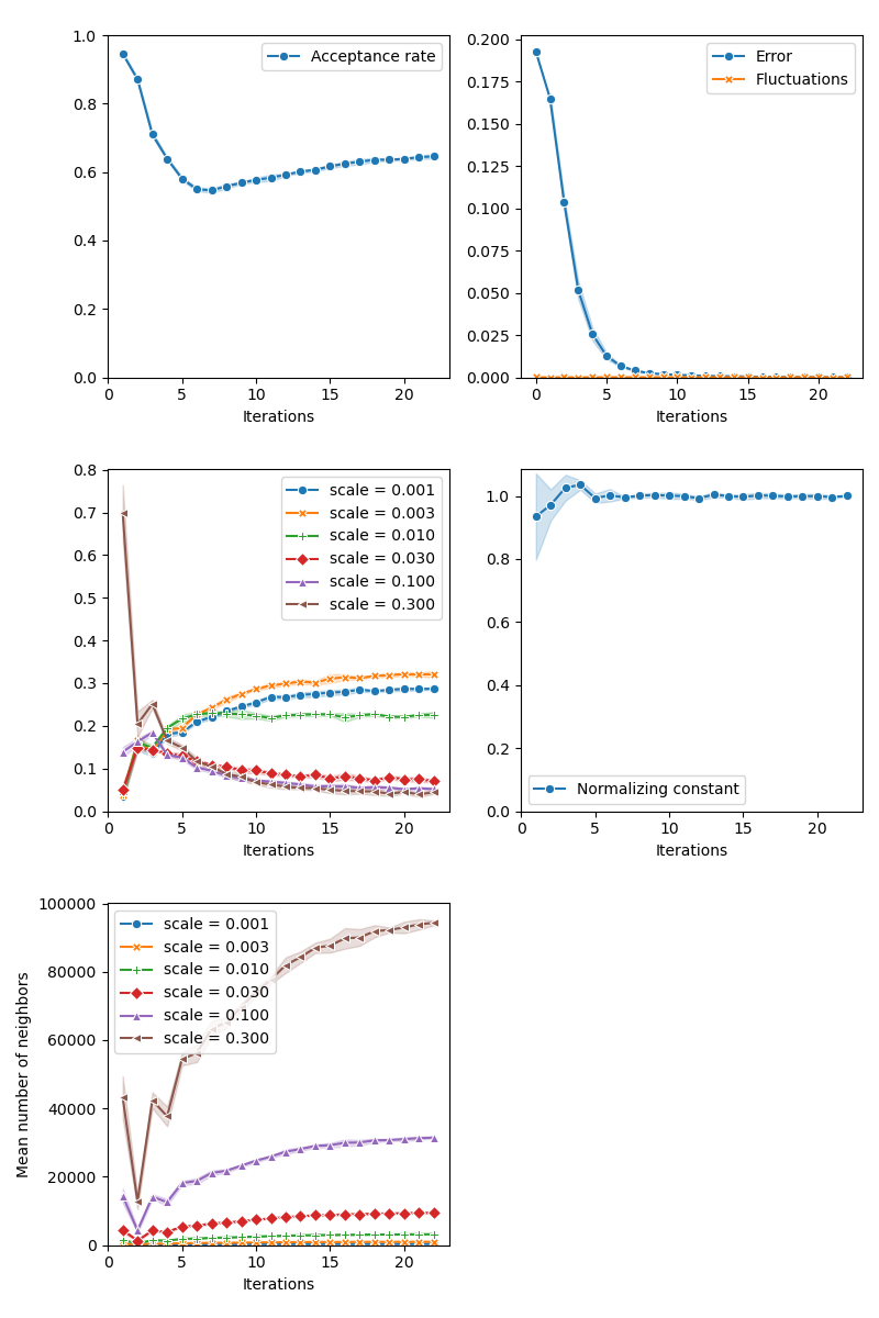
Our first algorithm - CMC with adaptive selection of the kernel bandwidth:

from monaco.samplers import MOKA_CMC

proposal = BallProposal(
    space,
    scale=[0.001, 0.003, 0.01, 0.03, 0.1, 0.3],
    exploration=exploration,
    exploration_proposal=exploration_proposal,
)
moka_sampler = MOKA_CMC(space, start, proposal, annealing=5).fit(distribution)
info["MOKA"] = display_samples(moka_sampler, iterations=20, runs=nruns)

• 
• 

With a Markovian selection of the kernel bandwidth:

from monaco.samplers import MOKA_Markov_CMC

proposal = BallProposal(
    space,
    scale=[0.001, 0.003, 0.01, 0.03, 0.1, 0.3],
    exploration=exploration,
    exploration_proposal=exploration_proposal,
)
moka_markov_sampler = MOKA_Markov_CMC(space, start, proposal, annealing=5).fit(
    distribution
)
info["MOKA Markov"] = display_samples(moka_markov_sampler, iterations=20, runs=nruns)

• 
• 

Our second algorithm - CMC with Richardson-Lucy deconvolution:

from monaco.samplers import KIDS_CMC

proposal = BallProposal(
    space,
    scale=[0.001, 0.003, 0.01, 0.03, 0.1, 0.3],
    exploration=exploration,
    exploration_proposal=exploration_proposal,
)
kids_sampler = KIDS_CMC(space, start, proposal, annealing=5, iterations=30).fit(
    distribution
)
info["KIDS"] = display_samples(kids_sampler, iterations=20, runs=nruns)

• 
• 

Combining bandwith estimation and deconvolution with the Moka-Kids-CMC sampler:

from monaco.samplers import MOKA_KIDS_CMC

proposal = BallProposal(
    space,
    scale=[0.001, 0.003, 0.01, 0.03, 0.1, 0.3],
    exploration=exploration,
    exploration_proposal=exploration_proposal,
)

kids_sampler = MOKA_KIDS_CMC(space, start, proposal, annealing=5, iterations=30).fit(
    distribution
)
info["MOKA+KIDS"] = display_samples(kids_sampler, iterations=20, runs=nruns)

• 
• 

Finally, the Non Parametric Adaptive Importance Sampler, an efficient non-Markovian method with an extensive memory usage:

from monaco.samplers import SAIS

proposal = BallProposal(
    space, scale=0.1, exploration=exploration, exploration_proposal=exploration_proposal
)


class Q_0(object):
    def __init__(self):
        self.w_1 = Nlucky / N
        self.w_0 = 1 - self.w_1

    def sample(self, n):
        nlucky = int(n * (Nlucky / N))
        x0 = 0.05 + 0.1 * torch.rand(n, D).type(dtype)
        x0[:nlucky] = 0.9 + 0.001 * torch.rand(nlucky, D).type(dtype)

        return x0

    def potential(self, x):
        v = 100000 * torch.ones(len(x), 1).type_as(x)
        v[(0.05 <= x) & (x < 0.15)] = -np.log(self.w_0 / 0.1)
        v[(0.9 <= x) & (x < 0.901)] = -np.log(self.w_1 / 0.001)
        return v.view(-1)


q0 = Q_0()

sais_sampler = SAIS(space, start, proposal, annealing=5, q0=q0, N=N).fit(distribution)
info["SAIS"] = display_samples(sais_sampler, iterations=20, runs=nruns)

• 
• 

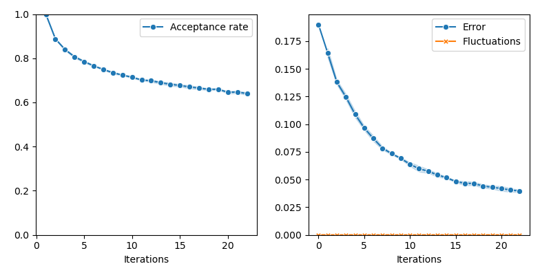
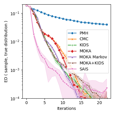
Comparative benchmark:

import itertools
import seaborn as sns

iters = info["PMH"]["iteration"]


def display_line(key, marker):
    sns.lineplot(
        x=info[key]["iteration"],
        y=info[key]["error"],
        label=key,
        marker=marker,
        markersize=6,
        ci="sd",
    )


plt.figure(figsize=(4, 4))
markers = itertools.cycle(("o", "X", "P", "D", "^", "<", "v", ">", "*"))

for key, marker in zip(
    ["PMH", "CMC", "KIDS", "MOKA", "MOKA Markov", "MOKA+KIDS", "SAIS"], markers
):
    display_line(key, marker)


plt.xlabel("Iterations")
plt.ylabel("ED ( sample, true distribution )")
plt.ylim(bottom=1e-4)
plt.yscale("log")

plt.tight_layout()


plt.show()