Note
Go to the end to download the full example code
Linking KeOps with scipy.sparse.linalg
The scipy library provides a simple abstraction for implicit tensors: the LinearOperator class, which represents generic “Matrix-Vector” products and can be plugged seamlessly in a large collection of linear algebra routines.
Crucially, KeOps pykeops.torch.LazyTensor are now fully compatible
with this interface.
As an example, let’s see how to combine KeOps with a
fast eigenproblem solver
to compute spectral coordinates on a large 2D or 3D point cloud.
Note
Ideally, we’d like to interface KeOps with some methods of the scikit-learn library… But this seems out of reach, as most of the sklearn codebase relies internally on explicit numpy arrays. One day, maybe!
Setup
Standard imports:
import matplotlib.pyplot as plt
import numpy as np

# noinspection PyUnresolvedReferences
from mpl_toolkits.mplot3d import Axes3D  # noqa: F401 unused import

from pykeops.numpy import LazyTensor
import pykeops.config

dtype = "float32"  # No need for double precision here!
Create a toy dataset, a spiral in 2D sampled with 10,000 points:
N = 10000 if pykeops.config.gpu_available else 1000
t = np.linspace(0, 2 * np.pi, N + 1)[:-1]
x = np.stack((0.4 + 0.4 * (t / 7) * np.cos(t), 0.5 + 0.3 * np.sin(t)), 1)
x = x + 0.01 * np.random.randn(*x.shape)
x = x.astype(dtype)
And display it:
plt.figure(figsize=(8, 8))
plt.scatter(x[:, 0], x[:, 1], s=5000 / len(x))
plt.axis("equal")
plt.axis([0, 1, 0, 1])
plt.tight_layout()
plt.show()
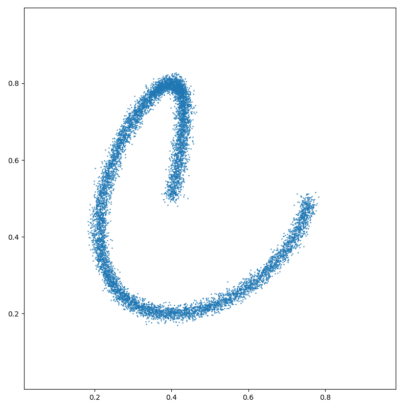
Ignoring fixed y limits to fulfill fixed data aspect with adjustable data limits.
Spectral coordinates
To showcase the potential of the KeOps-SciPy interface, we now perform spectral analysis on the point cloud x. As summarized by the Wikipedia page on spectral clustering, spectral coordinates can be defined as the eigenvectors associated to the smallest eigenvalues of a graph Laplacian.
When no explicit adjacency matrix is available, a simple choice is to use a soft kernel matrix such as the Gaussian RBF matrix:
which puts a smooth link between neighboring points at scale \(\sigma\).
sigma = 0.05
x_ = x / sigma
x_i, x_j = LazyTensor(x_[:, None, :]), LazyTensor(x_[None, :, :])
K_xx = (-((x_i - x_j) ** 2).sum(2) / 2).exp()  # Symbolic (N,N) Gaussian kernel matrix

print(K_xx)
KeOps LazyTensor
    formula: Exp((Minus(Sum(Square((Var(0,2,0) - Var(1,2,1))))) / IntCst(2)))
    shape: (10000, 10000)
Linear operators
As far as scipy is concerned, a KeOps pykeops.torch.LazyTensor such
as K_xx can be directly understood as a
LinearOperator:
from scipy.sparse.linalg import aslinearoperator

K = aslinearoperator(K_xx)
Just like regular numpy arrays or KeOps pykeops.torch.LazyTensor,
LinearOperators fully support the “matrix” product operator @.
For instance, to compute the mass coefficients
we can simply write:
D = K @ np.ones(N, dtype=dtype) # Sum along the lines of the adjacency matrix
Going further, robust and efficient routines such as eigsh can be used to compute the largest (or smallest) eigenvalues of our kernel matrix K at a reasonable computational cost:
from scipy.sparse.linalg import eigsh

eigenvalues, eigenvectors = eigsh(K, k=5)  # Largest 5 eigenvalues/vectors

print("Largest eigenvalues:", eigenvalues)
print("Eigenvectors of shape:", eigenvectors.shape)
Largest eigenvalues: [ 627.37     640.7966   665.13995  751.59546 1435.855  ]
Eigenvectors of shape: (10000, 5)
Graph Laplacian
Most importantly, LinearOperators can be composed
or added with each other.
To define our implicit graph Laplacian matrix:
we can simply type:
from scipy.sparse import diags

L = aslinearoperator(diags(D)) - K
L.dtype = np.dtype(
    dtype
)  # Scipy Bugfix: by default, "-" removes the dtype information...
Alternatively, we can also use a symmetric, normalized Laplacian matrix defined through:
D_2 = aslinearoperator(diags(1 / np.sqrt(D)))
L_norm = aslinearoperator(diags(np.ones_like(D))) - D_2 @ K @ D_2
L_norm.dtype = np.dtype(
    dtype
)  # Scipy Bugfix: by default, "-" removes the dtype information...
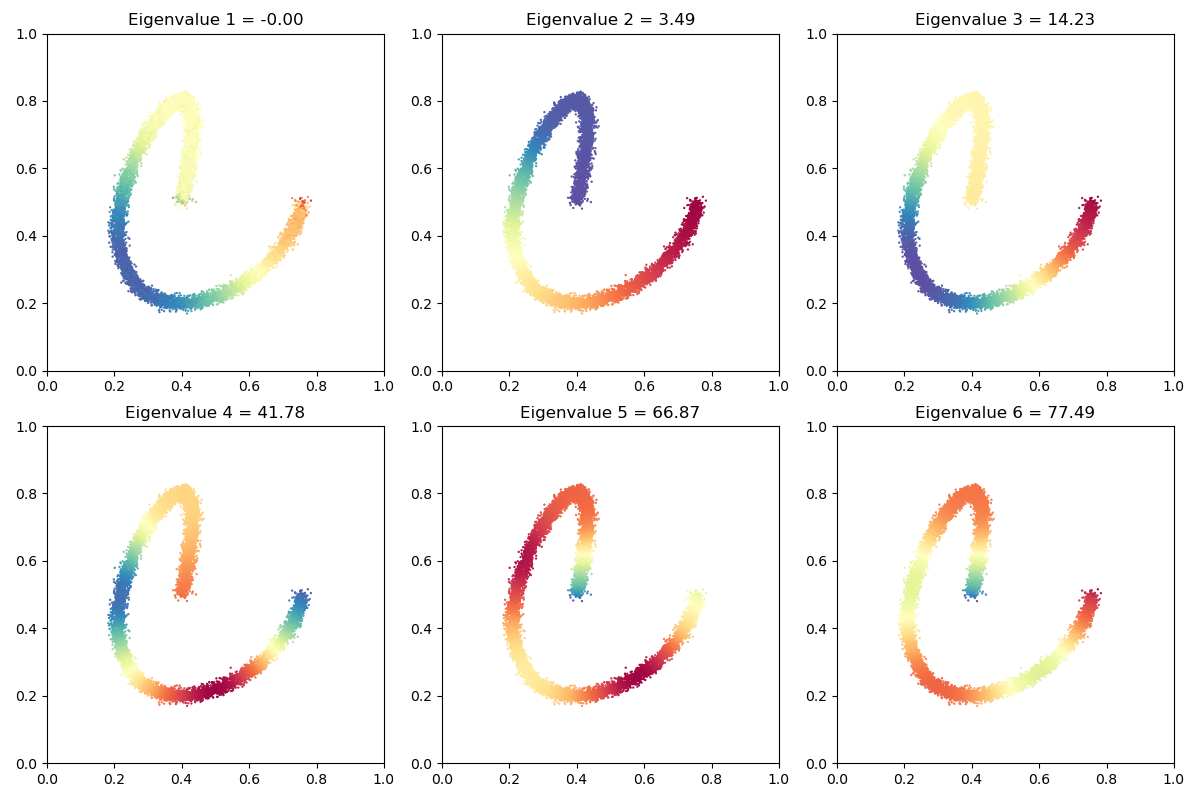
Then, computing spectral coordinates on x is as simple as typing:
from time import time

start = time()

# Compute the 7 smallest eigenvalues/vectors of our graph Laplacian
eigenvalues, coordinates = eigsh(L, k=7, which="SM")

print(
    "Smallest eigenvalues of the graph Laplacian, computed in {:.3f}s:".format(
        time() - start
    )
)
print(eigenvalues)
Smallest eigenvalues of the graph Laplacian, computed in 0.067s:
[-2.0990775e-04  3.4853592e+00  1.4165602e+01  4.1618130e+01
  6.7398979e+01  7.7885872e+01  1.1665987e+02]
That’s it! As expected, our first eigenvalue is equal to 0, up to the convergence of the Lanczos-like algorithm used internally by eigsh. The spectral coordinates, associated to the smallest positive eigenvalues of our graph Laplacian, can then be displayed as signals on the raw point cloud x and be used to perform spectral clustering, shape matching or whatever’s relevant!
_, axarr = plt.subplots(nrows=2, ncols=3, figsize=(12, 8))

for i in range(2):
    for j in range(3):
        axarr[i][j].scatter(
            x[:, 0],
            x[:, 1],
            c=coordinates[:, 3 * i + j],
            cmap=plt.cm.Spectral,
            s=9 * 500 / len(x),
        )
        axarr[i][j].set_title(
            "Eigenvalue {} = {:.2f}".format(3 * i + j + 1, eigenvalues[3 * i + j])
        )
        axarr[i][j].set_aspect("equal")
        axarr[i][j].set_xlim(0, 1)
        axarr[i][j].set_ylim(0, 1)

plt.tight_layout()
plt.show()
Scaling up to large datasets with block-sparse matrices
Going further, pykeops.torch.LazyTensor support
adaptive block-sparsity patterns (specified through an optional .ranges attribute)
which allow us to perform large matrix-vector products with sub-quadratic complexity.
To illustrate this advanced feature of KeOps,
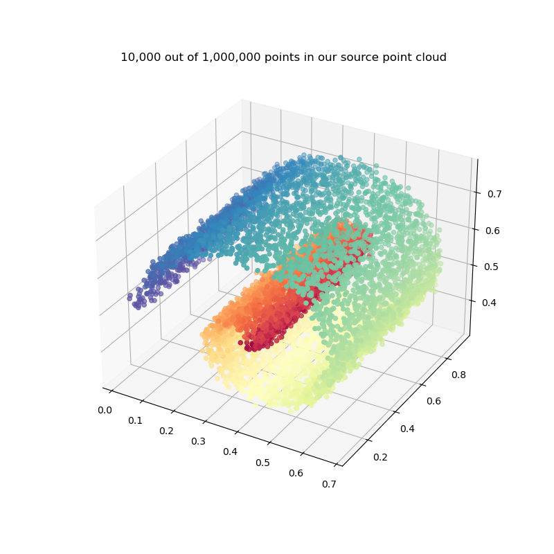
let’s generate a large “noisy Swiss roll” with 1,000,000 points in the unit cube:
N = 1000000 if pykeops.config.gpu_available else 1000
t = np.linspace(0, 2 * np.pi, N + 1)[:-1]
x = np.stack(
    (
        0.4 + 0.4 * (t / 7) * np.cos(1.5 * t),
        0.1 + 0.8 * np.random.rand(N),
        0.5 + 0.3 * (t / 7) * np.sin(1.5 * t),
    ),
    1,
)
x = x + 0.01 * np.random.randn(*x.shape)
x = x.astype(dtype)
To display our toy dataset with the (not-so-efficient) PyPlot library, we pick 10,000 points at random:
N_display = 10000 if pykeops.config.gpu_available else N
indices_display = np.random.randint(0, N, N_display)

_, ax = plt.subplots(nrows=1, ncols=1, figsize=(8, 8), subplot_kw=dict(projection="3d"))
x_ = x[indices_display, :]
ax.scatter3D(x_[:, 0], x_[:, 1], x_[:, 2], c=t[indices_display], cmap=plt.cm.Spectral)
ax.set_title("{:,} out of {:,} points in our source point cloud".format(N_display, N))
plt.show()
Can we scale the spectral analysis presented above to this huge dataset?
In practice, the radius \(\sigma\) of our kernel “adjacency” function is often much smaller than the diameter of the input point cloud: spectral methods rely on small-range neighborhoods to build a global coordinate system. Since \(k(x,y) \simeq 0\) above a threshold of, say, \(4\sigma\), a simple way of accelerating the kernel-vector product \(v\mapsto K_{xx}v\) in the (soft-)graph Laplacian is thus to skip computations between pairs of points that are far away from each other.
As explained in the documentation, fast GPU routines rely heavily on memory contiguity: before going any further, we must sort our input dataset to make sure that neighboring points are stored next to each other on the device memory. As detailed in the KeOps+NumPy tutorial on block-sparse reductions, a simple way of doing so is to write:
# Import the KeOps helper routines for block-sparse reductions:
from pykeops.numpy.cluster import (
    grid_cluster,
    cluster_ranges_centroids,
    sort_clusters,
    from_matrix,
)

# Put our points in cubic bins of size eps, as we compute a vector of class labels:
eps = 0.05
x_labels = grid_cluster(x, eps)
# Compute the memory footprint and centroid of each of those non-empty "cubic" clusters:
x_ranges, x_centroids, _ = cluster_ranges_centroids(x, x_labels)
# Sort our dataset according to the vector of labels:
x, x_labels = sort_clusters(x, x_labels)
Note
In higher-dimensional settings, the simplistic
grid_cluster
scheme could be replaced by a more versatile routine such as
our KeOps+NumPy K-means implementation.
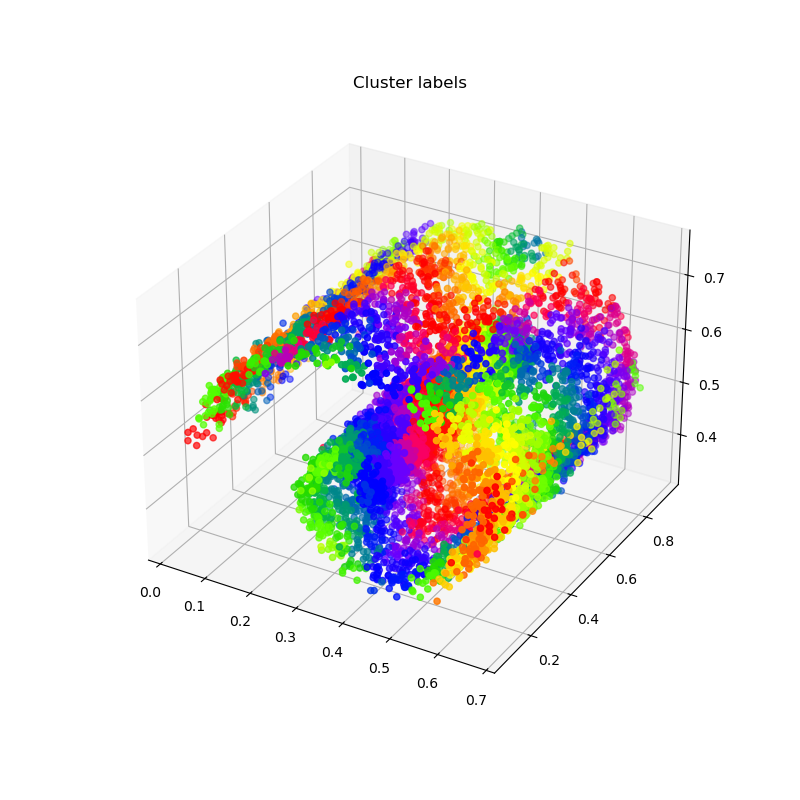
Points are now roughly sorted according to their locations, with each cluster corresponding to a contiguous slice of the (sorted) x array:
_, ax = plt.subplots(nrows=1, ncols=1, figsize=(8, 8), subplot_kw=dict(projection="3d"))
x_ = x[indices_display, :]
ax.scatter3D(x_[:, 0], x_[:, 1], x_[:, 2], c=x_labels[indices_display], cmap="prism")
ax.set_title("Cluster labels")
plt.show()
We can prune computations out of the \(v\mapsto K_{xx} v\) matrix-vector product in a GPU-friendly way by skipping whole blocks of cluster-cluster interactions. A good rule of thumb is to only consider pairs of points belonging to clusters \(X\) and \(Y\) whose centroids \(x_c\) and \(y_c\) are such that:
Considering that our cubic bins of size \(\varepsilon\) all have a diameter that is equal to \(\sqrt{3}\,\varepsilon\), this “block-sparsity” pattern can be encoded in a small boolean matrix keep computed through:
sigma = (
    0.01 if pykeops.config.gpu_available else 0.1
)  # Standard deviation of our Gaussian kernel
# Compute a coarse Boolean mask:
D = np.sum((x_centroids[:, None, :] - x_centroids[None, :, :]) ** 2, 2)
keep = D < (4 * sigma + np.sqrt(3) * eps) ** 2
which can then be converted to a GPU-friendly,
LIL-like sparsity pattern
with the from_matrix helper:
ranges_ij = from_matrix(x_ranges, x_ranges, keep)
Now, leveraging this information with KeOps is as simple as typing:
x_ = x / sigma  # N.B.: x is a **sorted** list of points
x_i, x_j = LazyTensor(x_[:, None, :]), LazyTensor(x_[None, :, :])
K_xx = (-((x_i - x_j) ** 2).sum(2) / 2).exp()  # Symbolic (N,N) Gaussian kernel matrix

K_xx.ranges = ranges_ij  # block-sparsity pattern
print(K_xx)
KeOps LazyTensor
    formula: Exp((Minus(Sum(Square((Var(0,3,0) - Var(1,3,1))))) / IntCst(2)))
    shape: (1000000, 1000000)
A straightforward computation shows that our new
block-sparse operator may be up to 20 times more efficient than a
full KeOps pykeops.torch.LazyTensor:
# Compute the area of each rectangle "cluster-cluster" tile in the full kernel matrix:
areas = (x_ranges[:, 1] - x_ranges[:, 0])[:, None] * (x_ranges[:, 1] - x_ranges[:, 0])[
    None, :
]
total_area = np.sum(areas)  # should be equal to N**2 = 1e12
sparse_area = np.sum(areas[keep])

print(
    "We keep {:.2e}/{:.2e} = {:2d}% of the original kernel matrix.".format(
        sparse_area, total_area, int(100 * sparse_area / total_area)
    )
)
We keep 5.19e+10/1.00e+12 = 5% of the original kernel matrix.
Good. Once we’re done with these pre-processing steps,
block-sparse pykeops.torch.LazyTensor are just as easy to interface with scipy as
regular NumPy arrays:
K = aslinearoperator(K_xx)
The normalized graph Laplacian can be defined as usual:
D = K @ np.ones(N, dtype=dtype)  # Sum along the lines of the adjacency matrix
D_2 = aslinearoperator(diags(1 / np.sqrt(D)))
L_norm = aslinearoperator(diags(np.ones_like(D))) - D_2 @ K @ D_2
L_norm.dtype = np.dtype(
    dtype
)  # Scipy Bugfix: by default, "-" removes the dtype information...
And our favourite solver will compute, as expected, the smallest eigenvalues of this custom operator:
from time import time

start = time()

# Compute the 7 smallest eigenvalues/vectors of our normalized graph Laplacian
eigenvalues, coordinates = eigsh(L_norm, k=7, which="SM")

print(
    "Smallest eigenvalues of the normalized graph Laplacian, computed in {:.3f}s ".format(
        time() - start
    )
    + "on a cloud of {:,} points in dimension {}:".format(x.shape[0], x.shape[1])
)
print(eigenvalues)
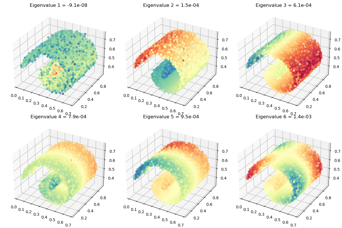
Smallest eigenvalues of the normalized graph Laplacian, computed in 48.665s on a cloud of 1,000,000 points in dimension 3:
[-6.7499002e-08  1.5505464e-04  6.1112683e-04  7.9273555e-04
  9.3856774e-04  1.3973579e-03  1.9836235e-03]
Note
On very large problems, a custom eigenproblem solver implemented with the PyTorch+KeOps interface should be sensibly faster than this SciPy wrapper: performing all computations on the GPU would allow us to perform linear operations in parallel and to skip hundreds of unnecessary Host-Device memory transfers.
Anyway. Displayed on a subsampled point cloud (for the sake of efficiency), our spectral coordinates look good!
x_ = x[indices_display, :]

# sphinx_gallery_thumbnail_number = 5
_, axarr = plt.subplots(
    nrows=2, ncols=3, figsize=(12, 8), subplot_kw=dict(projection="3d")
)

for i in range(2):
    for j in range(3):
        axarr[i][j].scatter3D(
            x_[:, 0],
            x_[:, 1],
            x_[:, 2],
            c=coordinates[indices_display, 3 * i + j],
            cmap=plt.cm.Spectral,
        )
        axarr[i][j].set_title(
            "Eigenvalue {} = {:.1e}".format(3 * i + j + 1, eigenvalues[3 * i + j])
        )

plt.tight_layout()
plt.show()
Total running time of the script: (0 minutes 52.554 seconds)