Note
Go to the end to download the full example code
Vectorial LogSumExp reduction
Let’s compute the (3000,1) tensor \(c\) whose entries \(c_i\) are given by:
where
\(x\) is a (3000,1) tensor, with entries \(x_i\).
\(y\) is a (5000,1) tensor, with entries \(y_j\).
\(a\) is a (5000,1) tensor, with entries \(a_j\).
\(p\) is a scalar, encoded as a vector of size (1,).
\(b\) is a (5000,3) tensor, with entries \(b_j\).
Setup
Standard imports:
import time

import matplotlib.pyplot as plt
import torch
from torch.autograd import grad

from pykeops.torch import Genred
Declare random inputs:
M = 3000
N = 5000

dtype = "float32"  # Could be 'float32' or 'float64'
torchtype = torch.float32 if dtype == "float32" else torch.float64

x = torch.rand(M, 1, dtype=torchtype)
y = torch.rand(N, 1, dtype=torchtype, requires_grad=True)
a = torch.rand(N, 1, dtype=torchtype)
p = torch.rand(1, dtype=torchtype)
b = torch.rand(N, 3, dtype=torchtype)
Define a custom formula
formula = "Square(p-a)*Exp(x+y)"
formula2 = "b"
variables = [
    "x = Vi(1)",  # First arg   : i-variable, of size 1 (scalar)
    "y = Vj(1)",  # Second arg  : j-variable, of size 1 (scalar)
    "a = Vj(1)",  # Third arg   : j-variable, of size 1 (scalar)
    "p = Pm(1)",  # Fourth arg  : Parameter,  of size 1 (scalar)
    "b = Vj(3)",
]  # Fifth arg   : j-variable, of size 3 (vector)

start = time.time()
Our log-sum-exp reduction is performed over the index \(j\),
i.e. on the axis 1 of the kernel matrix.
The output c is an \(x\)-variable indexed by \(i\).
my_routine = Genred(
    formula, variables, reduction_op="LogSumExp", axis=1, dtype=dtype, formula2=formula2
)
c = my_routine(x, y, a, p, b, backend="CPU")

# N.B.: By specifying backend='CPU', we can make sure that the result is computed using a simple C++ for loop.
print(
    "Time to compute the convolution operation on the cpu: ",
    round(time.time() - start, 5),
    "s",
    end=" ",
)
Time to compute the convolution operation on the cpu: 0.05525 s
We compare with the unstable, naive computation “Log of Sum of Exp”:
my_routine2 = Genred(
    "Exp(" + formula + ")*" + formula2,
    variables,
    reduction_op="Sum",
    axis=1,
    dtype=dtype,
)
c2 = torch.log(my_routine2(x, y, a, p, b, backend="CPU"))
print("(relative error: ", ((c2 - c).norm() / c.norm()).item(), ")")

# Plot the results next to each other:
for i in range(3):
    plt.subplot(3, 1, i + 1)
    plt.plot(c.detach().cpu().numpy()[:40, i], "-", label="KeOps - Stable")
    plt.plot(c2.detach().cpu().numpy()[:40, i], "--", label="KeOps - Unstable")
    plt.legend(loc="lower right")
plt.tight_layout()
plt.show()
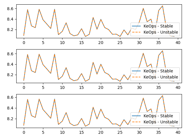
(relative error: 5.1402359702024114e-08 )
Compute the gradient
Now, let’s compute the gradient of \(c\) with respect to \(y\). Since \(c\) is not scalar valued, its “gradient” \(\partial c\) should be understood as the adjoint of the differential operator, i.e. as the linear operator that:
takes as input a new tensor \(e\) with the shape of \(c\)
outputs a tensor \(g\) with the shape of \(y\)
such that for all variation \(\delta y\) of \(y\) we have:
Backpropagation is all about computing the tensor \(g=\partial c . e\) efficiently, for arbitrary values of \(e\):
# Declare a new tensor of shape (M,1) used as the input of the gradient operator.
# It can be understood as a "gradient with respect to the output c"
# and is thus called "grad_output" in the documentation of PyTorch.
e = torch.rand_like(c)
# Call the gradient op:
start = time.time()
g = grad(c, y, e)[0]
# PyTorch remark : grad(c, y, e) alone outputs a length 1 tuple, hence the need for [0] at the end.

print(
    "Time to compute gradient of convolution operation on the cpu: ",
    round(time.time() - start, 5),
    "s",
    end=" ",
)
Time to compute gradient of convolution operation on the cpu: 0.03911 s
We compare with gradient of Log of Sum of Exp:
g2 = grad(c2, y, e)[0]
print("(relative error: ", ((g2 - g).norm() / g.norm()).item(), ")")


# Plot the results next to each other:
plt.plot(g.detach().cpu().numpy()[:40], "-", label="KeOps - Stable")
plt.plot(g2.detach().cpu().numpy()[:40], "--", label="KeOps - Unstable")
plt.legend(loc="lower right")
plt.tight_layout()
plt.show()
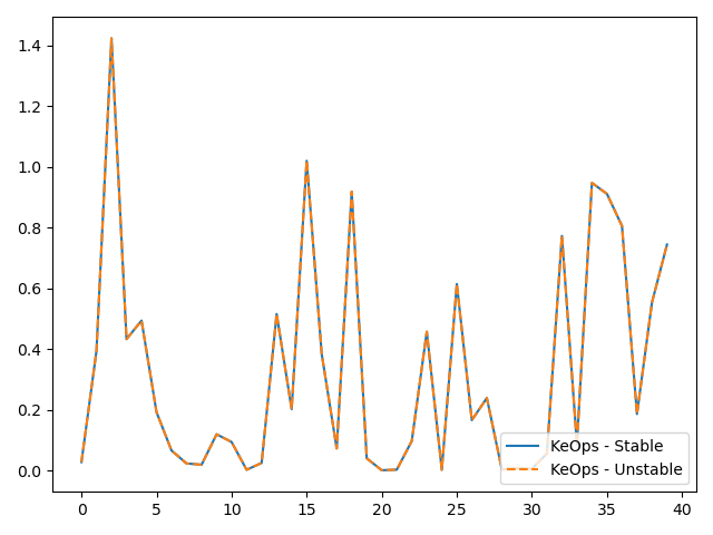
(relative error: 6.418613907044346e-08 )
Same operations performed on the Gpu
Of course, this will only work if you own a Gpu…
if torch.cuda.is_available():
    # first transfer data on gpu
    pc, ac, xc, yc, bc, ec = p.cuda(), a.cuda(), x.cuda(), y.cuda(), b.cuda(), e.cuda()
    # then call the operations
    start = time.time()
    c3 = my_routine(xc, yc, ac, pc, bc, backend="GPU")
    print(
        "Time to compute convolution operation on the gpu:",
        round(time.time() - start, 5),
        "s ",
        end="",
    )
    print("(relative error:", float(torch.abs((c2 - c3.cpu()) / c2).mean()), ")")
    start = time.time()
    g3 = grad(c3, yc, ec)[0]
    print(
        "Time to compute gradient of convolution operation on the gpu:",
        round(time.time() - start, 5),
        "s ",
        end="",
    )
    print("(relative error:", float(torch.abs((g2 - g3.cpu()) / g2).mean()), ")")

    # Plot the results next to each other:
    for i in range(3):
        plt.subplot(3, 1, i + 1)
        plt.plot(c.detach().cpu().numpy()[:40, i], "-", label="KeOps - CPU")
        plt.plot(c3.detach().cpu().numpy()[:40, i], "--", label="KeOps - GPU")
        plt.legend(loc="lower right")
    plt.tight_layout()
    plt.show()

    # Plot the results next to each other:
    plt.plot(g.detach().cpu().numpy()[:40], "-", label="KeOps - CPU")
    plt.plot(g3.detach().cpu().numpy()[:40], "--", label="KeOps - GPU")
    plt.legend(loc="lower right")
    plt.tight_layout()
    plt.show()
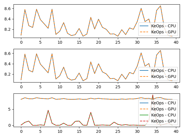
Time to compute convolution operation on the gpu: 0.00074 s (relative error: 2.1681474393631106e-08 )
Time to compute gradient of convolution operation on the gpu: 0.00096 s (relative error: 1.0918753901023592e-07 )
Total running time of the script: (0 minutes 0.618 seconds)