Tutorials, applications
These tutorials present real-life applications of the pykeops.numpy
and pykeops.torch modules,
from Gaussian processes to Optimal Transport theory and K-means clustering.
Note
If you run a KeOps script for the first time, the internal engine may take a few minutes to compile all the relevant formulas. Do not worry: this work is done once and for all as KeOps stores the resulting shared object files (‘.so’) in a cache directory.
KeOps 101: Working with LazyTensors
Thanks to the pykeops.numpy.LazyTensor and pykeops.torch.LazyTensor decorator,
KeOps can now speed-up your
NumPy or PyTorch programs without any overhead.


Using KeOps as a backend
KeOps can provide efficient GPU routines for high-level libraries such as scipy or GPytorch: if you’d like to see tutorials with other frameworks, please let us know.


Gaussian Mixture Models
KeOps can be used to fit Mixture Models with custom priors on large datasets:

Interpolation - Splines
Thanks to a simple conjugate gradient solver,
the numpy.KernelSolve and torch.KernelSolve
operators can be used to solve large-scale interpolation problems
with a linear memory footprint.


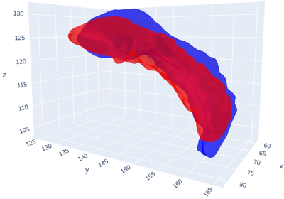
Kernel MMDs, Optimal Transport
Thanks to its support of the Sum and LogSumExp reductions, KeOps is perfectly suited to the large-scale computation of Kernel norms and Sinkhorn divergences. Going further, the block-sparse routines allow us to implement genuine coarse-to-fine strategies that scale (almost) linearly with the number of samples, as advocated in (Schmitzer, 2016).
Relying on the KeOps routines generic_sum() and
generic_logsumexp(),
the GeomLoss library
provides Geometric Loss functions as simple PyTorch layers,
with a fully-fledged gallery of examples.
Implemented on the GPU for the very first time, these routines
outperform the standard Sinkhorn algorithm by a factor 50-100
and redefine the state-of-the-art
for discrete Optimal Transport: on modern hardware,
Wasserstein distances between clouds of 100,000 points can now be
computed in less than a second.